Nick Rowe has a post entitled “AS/AD: A Suggested Interpretation”. I’m going to offer a very different interpretation, which (interestingly) has almost identical implications. I’m not quite sure why.
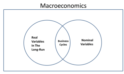
In my view, the “classical dichotomy” lies at the very heart of macroeconomics. It’s the central organizing principle:
This is the view that one set of factors determines nominal variables, and a completely different set of factors determines real variables. Both Nick and I agree that monetary factors are what determine nominal variables.
If that’s all one had to say about the classical dichotomy, then the AS/AD model might look something like this:
Monetary factors would determine the position of the AD curve, and hence the price level, but would leave real output unchanged. BTW, this view of things makes no assumptions about how the money supply or velocity change over time. It simply looks at the economy in terms of factors that determine nominal variables (AD) and factors that determine real magnitudes (position of long run aggregate supply.)
After teaching the classical dichotomy, textbooks usually explain that wages and prices are sticky, and hence that the classical dichotomy does not hold in the short run. That’s the overlap in the Venn Diagram above. But there’s no follow up; the textbooks don’t explain what any of that means. The chapter with MV=PY and the classical dichotomy and money neutrality just sort of drifts off into nowhere, like a Chinese river than ends up in the Taklamakan desert.
Instead, about 5 chapters later the textbook will start discussing a mysterious AS/AD model, which seems sort of like a S&D model, but is actually completely unrelated to supply and demand. Instead, the AS/AD model is finally explaining to students what we meant 5 chapters earlier when we talked about the classical dichotomy and money neutrality and sticky prices and MV=PY, but of course no student would see the connection—and why should they?
There’s a slightly better chance that students would understand what’s actually going on here if you called the AD curve the “nominal spending” (NS) curve, or even the MV line. Movements in the line (caused by M or V, it makes no difference) would be called “nominal shocks” not demand shocks. They have nothing to do with “demand” as the concept is taught in microeconomics, but the unfortunate terminology explains why so many people (wrongly) think that “if consumers sit on their wallets then aggregate demand will decline”. In fact, sitting on your wallet means saving, and saving equals investment, and attempts to save will reduce interest rates which might reduce velocity, which could reduce AD, except it won’t because the central bank targets inflation . . . or something like that.
Then the Short Run Aggregate Supply curve would be introduced. Students would be told that the purpose of the SRAS curve is to show how (because of sticky wages) nominal shocks are partitioned into a change in both output and prices, in the short run. (Long run money neutrality is still assumed.)
I don’t have quite as strong an objection to calling the SRAS curve a “supply curve” as I prefer the sticky wage version of AS/AD, which is the version where the term ‘supply’ fits best. But as a favor to those that don’t like the sticky wage version, it might be better to give it a different name, such as the “real output” (RO) line. If you believe in sticky prices, or money illusion, or misperceptions, then it’s not really a supply curve.
Thus the AS/AD model is simply a way of showing how nominal shocks have real effects in the short run, but the classical dichotomy holds in the long run. (David Glasner would quibble about the last point, so perhaps we could say monetary neutrality “almost” holds true in the long run.)
Even better would be if you introduced AS/AD immediately after discussing why the classical dichotomy holds in the short run but not the long run. All in one chapter. You dispense with the “three reasons the AD curve slopes downwards”, which almost no undergraduate understands.
If you read Nick’s post, his AS/AD explanation will seem totally different. And yet we both believe (AFAIK) almost the same things about real world monetary policy, optimal monetary policy, the way that interest rates confuse the issue, the subtle problems with new Keynesian and NeoFisherian theory, the not so subtle problems with MMT, and a dozen other practical monetary questions. One question for further study is how can we end up in almost the exact same place, after taking such different paths?
If you are having trouble contrasting our two views, keep in mind that Nick and I don’t disagree as to what the AD curve “really looks like”, we are describing totally different concepts. Thus to me, the curve Nick talks about isn’t what I think of AD at all, as it could theoretically slope upwards, which can never be true of a “nominal spending line” (which must be a downwards sloping hyperbola). His AD curve depends on the monetary regime, mine does not. In his model the economy can be temporarily “off the line”. In mine the economy is always at equilibrium, every single nanosecond, because the “RO” line is derived by looking at where the economy actually is, and the NS line is actual nominal spending.
In a strange way, however, the radically different nature of the two ways that we visualize AS/AD might help to answer the question I posed above. If we had the same conception of AD curves, but different versions, then our two models would surely have different real world implications. But they don’t seem to. Again, it seems like two radically different roads, leading to the same destination. Odd.
PS. In my version, it’s just as correct to call the NS line ‘aggregate supply’ as aggregate demand. In fact, it’s an equilibrium quantity, both “the quantity of nominal aggregate demand”, and “the quantity of nominal aggregate supply”. It’s merely NGDP.
READER COMMENTS
CB
Jan 21 2017 at 12:38pm
Hi,
Young Econ undergrad here: I’m slightly confused as to why you posited that a reduction in interest rates could reduce the velocity of money. Wouldn’t the price of money becoming “cheaper” (lower interest rates) raise the quantity demanded of money? Then, as people presumably demand and use more money, the amount of transactions taking place in an economy would increase. At least, according to my knowledge. If you could please explain what you meant, I’d appreciate it! Thanks.
Market Fiscalist
Jan 21 2017 at 12:45pm
If I had to pick a single chart that captures the essence of the economics I have learned from your (and Nick’s) blog it would be the second of the charts you show here. It captures excellently how (given a fixed M and V) actual NGDP is derived, and how when either M or V changes actual NGDP will change as a result of a shifting AD curve and a shift along the AS curve that reflects the way that suppliers react to a demand change by a combination of price and qty changes. The economy is always at the equilibrium point , it just may not be the full employment equilibrium. By extension anyone who control M can control NGDP by adjusting it in reaction to changes in V.
I think the only downside to your model is that all changes in M or V lead to the AD curve shifting left or right. I’m not sure I have fully grasped it yet but I think Nick’s model avoids this by having his AD and AS curves reflect all possible values of M and V that lead to desired and actual money flows being equal, and only one point (which would match your equilibrium point) where these flows are equal on both the demand and supply side. This means (as you say) that it is quite possible for actual AD and AS to be off both curves at any point in time if the economy is out of equilibrium on both curves. I am not yet convinced that the extra complexity of doing it this way adds sufficient value to justify the extra brain power needed to grasp it !
Iskander
Jan 21 2017 at 1:23pm
@CB,
The idea is that a lower interest rate reduces the opportunity cost of holding money, therefore increasing demand for money (ceteris paribus of course).
So the demand for money increases, meaning that people will not spend all of the money they receive, using what is not spent to top up their cash balances until they reach their target level. This means that the velocity of money has been reduced. (I think it helps to think of money as a hot potato, if the demand for money increases people hold onto money for a longer period of time, i.e reduced velocity)
MV=PY
Since V has declined, assuming that the money supply is constant, either P or Y must fall. In the long run P falls to fully account for the fall in V (long run neutrality of money), however since P is sticky in the short run, Y falls.
This is a simplified version of what I’ve picked up from Scott, Nick Rowe and Friedman.
From another undergrad (Apologies to all if I’m wrong anywhere).
Nick Rowe
Jan 21 2017 at 2:32pm
Scott: Hmmm. Yes, we do think of it very differently, but still end up in the same place. Which is a puzzle.
Let me try to resolve that puzzle by asking you this: suppose we are doing partial equilibrium micro. We *could*, if we wanted to, draw a rectangular hyperbola NS curve for a given level of nominal spending on apples. But it wouldn’t be very useful to draw it, and we would still need the standard demand curve to tell us what happens to NS if the supply curve shifts (or if the price of pears changes). Why is the NS curve more useful in macro than in partial equilibrium micro?
CB: Iksander has it right. You are thinking about the demand for a flow of loans, or borrowing money (which you will presumably plan to spend not hold). Scott (and me and Iksander) are talking about the average stock of money that people want to hold in their pockets and bank accounts; it’s like an inventory we need to hold so we don’t have to have exactly the same flow in and flow out at each second in time.
Don Geddis
Jan 21 2017 at 2:52pm
@CB, @Iskander: What makes this complicated, is that there are multiple things happening at the same time. Iskander is correct, that if interest rates are high, the opportunity cost of maintaining large cash balances is high, and so there is incentive to “get rid of” large cash balances (= hot potato effect), and thus velocity is high. As a consequence, if interest rates lower, then the opportunity pain of holding on to large cash balances lowers, and so more people do it, and velocity falls.
At the same time, CB asked about a scenario where there was a “reduction in interest rates”. The paragraph above was “all else equal” … but for interest rates to reduce, something else must be different. What is it? (This is Sumner’s “never reason from a price change”.) Probably CB is thinking of the central bank’s monetary policy causing interest rates to lower, by … increasing the money supply. (Please note: there are other ways to lower interest rates, some of which have the opposite consequences!)
So if MV=PY=NGDP, and we agree that lower interest rates reduce V, except we now hypothesize that you got the lower rates by increasing M, then you really don’t (yet) know whether NGDP is going to go up or down. Which may match CB’s intuition that the central bank caused interest rates to lower, and as a consequence overall spending rose. That’s a perfectly feasible scenario … but it happened because M rose, not because V did.
Pietro Poggi-Corradini
Jan 21 2017 at 5:30pm
Scott, can you please write an intro to macro text?
Lorenzo from Oz
Jan 21 2017 at 7:15pm
What he said. And, go for broke, use sensible terms rather than the inherited jargon misleads.
Lorenzo from Oz
Jan 21 2017 at 7:18pm
Or co-write one with Nick Rowe. And possibly David Glasner. (I know there are some disagreements between you, but think of it as productive tension.)
Scott Sumner
Jan 22 2017 at 12:21am
CB, Yes, it would increase the demand for money. An increase in money demand is a decrease in velocity. When you decrease money demand, that’s when spending goes up. Spending is a way to get rid of money.
Nick, Nominal shocks are not useful in micro, as what matters is relative (real) concepts. In macro, nominal shocks (or value of money shocks, if you prefer) are really important because they lead to disequilibrium in the labor market. That’s why you want to pay close attention to NGDP. It’s unexpected changes in NGDP that create macro instability, and the NS curve (combined with SRAS) is a good way to show this.
Pietro and Lorenzo, I’m working on it.
Comments are closed.