Forecasting and Econometric ModelsAbout the Author |

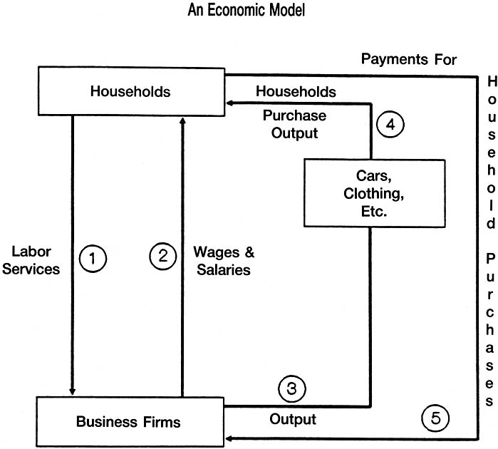
Before econometricians can make such calculations, they need what is called an economic model, or a theory of how different factors in the economy interact with one another. For instance, think of the economy as composed of households and business firms, as depicted on the left-hand side of figure 1. Households supply business firms with labor services (as tailors, accountants, engineers, etc.) and earn wages and salaries from the businesses in exchange for their labor. Using the labor services, businesses produce various outputs (clothing, cars, etc.), which are available for purchase (right-hand side of figure 1). Households, using the earnings derived from their labor services, become the customers who purchase the output. The products produced by the businesses wind up in the households, and the wage and salary payments return to the businesses in exchange for the products being sold to the households.

Figure 1. An Economic Model
Enlarge in new window
This chain of events, as shown by the activities numbered 1 through 5 in figure 1, is a description—or diagrammatic model—of the operation of a private enterprise economy. It is obviously incomplete. There is no central bank supplying money, no banking system, and no government levying taxes, building roads, or providing education. But the essentials of the private sector of the economy—working, producing, and buying products and services—are represented in a useful way in figure 1.
The diagrammatic model of figure 1 has certain disadvantages when it comes to representing quantities, such as the value of the wage and salary payments or the number of cars produced. To represent magnitudes more conveniently, economists employ a mathematical model, which basically is a set of equations that describe various relationships between variables. Consider household purchases of output, shown as activity number 4 in figure 1. If W is the amount of wages and salaries earned by households, and C is household expenditures on clothing, then the equation C = .12W states that households spend 12 percent of their wages and salaries on clothing. An equation could also be constructed to represent household purchases of cars or any other goods and services. Indeed, each of the activities pictured in figure 1 can be represented in the form of an equation. Doing so may take a blend of economic theory, physical and institutional realities, and mathematical sophistication, but once done, the result would be a mathematical or "quantitative economic model," which is but one important step away from an econometric model.
The equation for clothing purchases, C = .12W, asserts that 12 percent of household income is spent on clothing. That "12 percent" was selected purely for illustrative purposes. But if the model is to say anything useful about the American economy of today, the model must contain numbers (econometricians and others applying similar statistical methods refer to such numbers as parameters) that describe what really goes on in the real world. For this purpose one can turn to the relevant historical data to find out what percentage of household income Americans do, in fact, typically spend on clothing. Table 1 presents the figures for the years 1984 through 1989.
| TABLE 1
|
|
|
Spending on Clothing
|
|
| Year |
% of Household Income |
| 1984 | 5.8 |
| 1985 | 5.8 |
| 1986 | 6.0 |
| 1987 | 6.0 |
| 1988 | 5.9 |
| 1989 | 6.0 |
|
|
|
Obviously, the illustrative 12 percent figure was way off and, if left in the model, would have led to serious errors in application to the American economy. A more appropriate value is 5.9 percent, which implies the equation C = .059W. Because the parameter value of .059 in the clothing equation is derived from the relevant data, the equation should say something meaningful about the economy. Using real data to determine or estimate all the parameter values in the model is the critically important step that turns the abstract mathematical economic model into an econometric model.
An econometric model is said to be complete if it contains enough equations to predict values for all of the variables in the model, such as C and W. The single equation C = .059W, for example, predicts C if the value of W is known. Thus, there must be an equation somewhere in the model that determines W. If all such logical connections have been made, the model is complete and can, in principle, be used to forecast the economy or to test theories about its behavior.
Actually, no econometric model is ever truly complete. All models contain variables that the model cannot predict because they are determined by forces "outside" the model. For example, a realistic model must include personal income taxes collected by the government because taxes are the "wedge" between the gross income earned by households and the net income (what economists call disposable income) available for households to spend. The taxes collected depend on the tax rates in the income tax laws. If the model is to forecast economic activity several years into the future, anticipated future tax rates must be made a part of the model's information base. That requires an assumption about whether the government will change future income tax rates and, if so, when and by how much. Similarly, the model requires an assumption about the monetary policy that will be pursued by the central bank (the Federal Reserve System in the United States), and assumptions about many other such "outside of the model" (or exogenous) variables in order to forecast all the "inside of the model" (or endogenous) variables.
The need for the econometrician to use the best available economic judgment about "outside" factors is inherent in economic forecasting. An econometrically based economic forecast can, therefore, be wrong for several reasons:
-
1. incorrect assumptions about the "outside," or exogenous, variables, which are called input errors
2. econometric equations that are only approximations to the truth (note that clothing purchases do not amount to exactly 5.9 percent of household income every year), which are called model errors
3. some combination of input error and model error
Most econometric forecasters believe that economic judgment can and should be used not only to determine values for exogenous variables (an obvious requirement), but also to reduce the likely size of model error. Taken literally, the equation C = .059W means that "any deviation of clothing purchases from 5.9 percent of household income must be considered a random aberration from normal or expected behavior"—one of those inherently unpredictable vagaries of human behavior that continually trip up pollsters, economists, and any others who attempt to forecast socioeconomic events.
The economic forecaster must be prepared to be wrong because of unpredictable model error. But is all model error really unpredictable? Suppose the forecaster reads reports that indicate unusually favorable consumer reaction to the latest styles in clothing. Suppose that on this basis, the forecaster believes that about 6.5 percent of household income, rather than the usual 5.9 percent, will be spent on clothing next year. Should the forecaster ignore his belief that clothing sales are about to "take off," leave the model alone, and produce a forecast that he expects to be wrong?
The answer depends on the purpose of the forecast. If the purpose is the purely scientific one of determining how accurately a well-constructed model can forecast, the answer must be "Ignore the outside information and leave the model alone." If the purpose is the more pragmatic one of using the best available information to produce the most informative forecast, the answer must be "Incorporate the outside information into the model, even if that means effectively 'erasing' the parameter value .059 and replacing it with .065 while generating next year's forecast." Imposing such constant adjustments on forecasts used to be disparaged as entirely unscientific. In recent years, however, researchers have begun to regard such behavior as inevitable in the social science of economic forecasting and have begun to study how best—from a scientific perspective—to incorporate such outside information.
Much of the motivation behind trying to specify the most accurately descriptive economic model, trying to determine parameter values that most closely represent economic behavior, and combining these with the best available outside information arises from the desire to produce accurate forecasts. Unfortunately, the accuracy of an economic forecast is not easy to judge. There are simply too many dimensions of detail and interest. One user of the forecast may care mostly about gross national product (GNP), another mostly about exports and imports, and another mostly about inflation and interest rates. Thus, the same forecast may provide very useful information to some users, while being misleading to others.
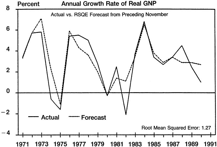
For want of anything obviously superior, the most common gauge of the quality of a forecast is how accurately it predicts real GNP. Real GNP is the most inclusive summary measure of total national production. For many purposes there is much value in knowing, with some lead time, whether to expect real GNP to be increasing rapidly (a booming economy), to be slowing down or speeding up relative to recent behavior, or to be declining (a slumping or recessionary economy). The information contained in chart 1 can be used to judge, in the summary fashion just indicated, the forecasting accuracy achieved by the econometric model I work on, that of the Research Seminar in Quantitative Economics (RSQE) of the University of Michigan.

Chart 1. RSQE Forecast Accuracy: 1971-1990
Enlarge in new window
The RSQE forecasting project, dating back to the fifties, is one of the oldest in the United States. Chart 1 compares, for each of the years from 1971 through 1990, the actual percent change in real GNP (the economy's growth rate) with the RSQE forecast published in November of the preceding year. Although the forecast missed the actual percentage change by an average of 1.27 percentage points, the forecast was sometimes off by considerably more than that—by 3.2 percentage points for 1982, for example. Nonetheless, there was never a boom year that RSQE forecast to be a bad year, never a bad year that RSQE forecast to be a boom year, and almost never an instance in which the forecast didn't provide the right information as to whether the economy's growth rate was about to speed up or slow down. These forecast errors would be large if we were forecasting a rocket trajectory. But economics is a social science with few truly reliable laws of behavior, and chart 1 surely is suggestive of a long record of informative GNP forecasting.
Econometric forecasting is the joint product of the econometric model and the economist who uses it. Studies have shown that forecasts that combine the model and the forecaster's judgment are generally more accurate than "purely objective" forecasts that are produced with the econometric model alone. Models are, however, routinely used by themselves in the important area of econometric policy analysis and in other "what if" calculations. Thus, a baseline forecast may be calculated using the model and the best information available to the forecaster. Then some question is asked, such as "What if the income tax rate is increased by 10 percentage points?" The forecaster puts the new tax rate into the model and recalculates the projected level of, say, real GNP, to show the new tax rate's effect on the economy.
Economists commonly employ such calculations to help them advise businesses and governments. The practical validity of such applications depends on how well the model's structure represents the economic behavior that is central to the "what if" question being asked. All models are merely approximations to reality; the issue is whether a given model's approximation is good enough for the question at hand. Thus, making models more accurate is important. As long as people ask "What if...?" econometric models will continue to be used and useful.
Saul H. Hymans is a professor of economics and statistics and director of the Research Seminar in Quantitative Economics at the University of Michigan.
Howrey, E. Philip, Saul H. Hymans, and Michael R. Donihue. "Merging Monthly and Quarterly Forecasts: Experience with MQEM." Journal of Forecasting 10 (May 1991): 255-68
Klein, Lawrence R., ed. Comparative Performance of U.S. Econometric Models. Especially chaps. 1, 3, 10, 11, 12. 1991.
Klein, Lawrence R., and Richard M. Young. An Introduction to Econometric Forecasting and Forecasting Models. 1980.

