The Common Sense of Political Economy
By Philip H. Wicksteed
Philip H. Wicksteed (1844-1927) wrote the
The Common Sense of Political Economy, Including a Study of the Human Basis of Economic Law (Macmillan and Co., Limited, St. Martin’s Street, London) in 1910.The edition presented here is the first edition, which was widely used as an economics textbook in classrooms in the United Kingdom and the United States, and probably elsewhere as well.A few corrections of obvious typos were made for this website edition. We also added occasional parentheses or square brackets to mathematical expressions for clarity [this was necessary in cases where the requirements of browsers to print fractions with a solidus (“/”) causes potential confusion when the entire fraction is to be multiplied by a subsequent factor:
e.g., to distinguish (1/2
x) versus (1/2)
x]. However, because the original edition was so internally consistent and carefully proofread, we have erred on the side of caution, allowing some typos to remain lest someone doing academic research wishes to follow up. We have changed some small caps to full caps for ease of using search engines.Editor
Library of Economics and Liberty
2000
First Pub. Date
1910
Publisher
London: Macmillan and Co.
Pub. Date
1910
Comments
1st edition.
Copyright
The text of this edition is in the public domain.
BUYER AND SELLER. DEMAND AND SUPPLY
CHAPTER IV
Summary.—
This chapter deals with the application of the diagrammatic method of curves to the phenomena of the market. Individual curves of price-and-quantity-taken, if properly constructed for the purpose, can be added into a communal curve, on which the price corresponding to any given supply can be read. A disguised method of reaching the same result by means of intersecting curves is frequently employed, but though legitimate in itself it is misleading when used, as it generally is, in conjunction with a distinction between buyers and sellers, which is irrelevant to the issue. The same principle that determines the flow of any given commodity to the various consumers also determines the flow of the factors of production to the different industries. Capacity for productive effort is distributed between economic and non-economic employments, or is reserved and not put forth at all, on the general principles of the distribution of resources or choice between alternatives.
We have seen that the curves of the total significance of different commodities to the same individual cannot be added together, though a joint curve of two or more commodities can be constructed independently. When we pass to the consideration of the summation of curves of different individuals referring to the same commodity, we see at once that so far as we interpret them psychologically there can be no sense in speaking of addition at all, for there is no common psychological unit. But so far as we interpret them as curves of quantity-taken-at-the-price, there seems no reason why they should not be added. If we know the quantity that each individual would take at a given price, we know the quantity that they would take amongst them, and if we know the total supply of the article, we can find the price by determining to what point of relative marginal significance that supply will satisfy all the individuals concurrently.
But here a difficulty presents itself. If the price rises because the supply is reduced, the amount that A will take at this higher price is affected by the terms on which he can get all the available substitutes; but if B is having his stock reduced at the same time as A he will probably run to the same substitutes, and since this will raise their market value A will find that the conditions under which he made his estimates have been violated. We asked him how much he would take at such a price, “all other things remaining equal,” and we constructed his curve from his replies; but now we find that (in the normal case) as the price rises all other things do not remain equal, for the price of substitutes rises also; and the modifications which this will introduce into A’s estimate of the relative significance (expressed in the objective unit) of the commodity at any given margin cannot be determined simply by analysing his present sense of values, for the terms on which the alternatives will be offered to him will be changed to an extent which he cannot determine and which does not depend on his own estimates of different satisfactions.
It is the dealer’s business to forecast the effect which a change in the supply will produce upon the price of the commodity when all these reactions have had their full effect, but he will not individualise the different demands. He will estimate the nature of the sum of all the individual curves, but he will think of it (or at any rate estimate it) as a single thing, not as arrived at by the addition of a number of individual demands. Thus, neither the mind of the dealer nor the minds of the individual consumers contain material out of which we could construct a number of personal curves of price-and-quantity-consumed, which could be added together into a total curve. The dealer’s mind contains the material for the (speculative) construction of such a total curve, but not for the construction of the elements out of which it is composed; and the minds of the individual consumers contain the material out of which the first approximation to the individual curves might be made, but not the material for estimating the modifications which will be produced in those individual curves by the reaction of the changing prices of substitutes, which the dealer estimates in the mass.
*28
Nevertheless, it remains true that these effects, which are only estimated by the dealer in the mass, are actually composed of the sum of the effects on individual demands, and we may therefore conceive ideally of a series of individual curves of price-and-quantity-demanded, in which these reactions have been discounted, and which can therefore be added together.
They will represent for each individual the prices which he would give for each successive increment sooner than go without it, under the modified possibilities as to substitutes which would accompany the contracted supply which caused the rise in price; and the sum of them will constitute a collective scale shewing at what price any given quantity of the commodity could be sold, or what quantity could be sold at any given price, all other supplies remaining constant, though the demand upon those other supplies varies.
In
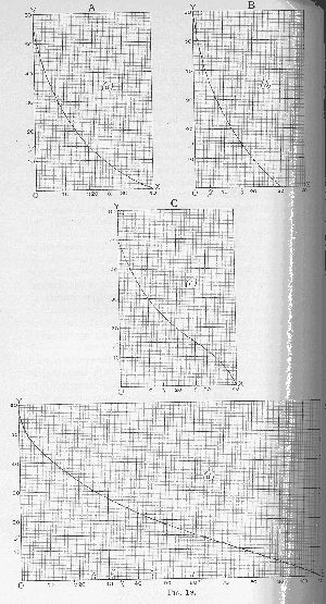 Fig. 19 let (
a), (
b), (
c), etc., represent the curves of one commodity for the individuals A, B, C, etc. On the axis of X the commodity itself is measured in its proper conventional unit, and on the axis of Y the corresponding price or marginal significance is marked. Now take (
d) equal to the sum of (
a), (
b), and (
c) read laterally. That is to say, for any ordinate of determined length
Oy the abscissa on (
d) is to equal the sum of the abscissas on (
a), (
b), and (
c).
Supposing A, B, and C to represent all the potential consumers of the commodity, this would mean that (
d) represents its collective or communal scale of significance. If we have the three curves and know the total amount of the commodity at command, we can construct the collective curve (
d), measure off the total supply on its abscissa, as
Ox, and find the corresponding ordinate
Oy. This will be the point of relative significance down to which all the claimants will be satisfied; and we can measure off the several abscissas on (
a), (
b), and (
c) that it will determine. They will shew the amounts of the commodity that A, B, and C will respectively take out of the market. The communal curve will be represented by (
d), on which equal areas, though they represent satisfactions that correspond to the same objective unit, have not the same psychological significance.
This addition of curves is given primarily as a graphic device for finding that point on the ordinates of the curves which will make the corresponding abscissas amount, in their sum, to the total supply. This distribution is actually determined by the play of the demands represented by the several curves. If the supply were distributed in any other way, there would be no equilibrium, and the conditions of further exchange would exist. But we have seen that the collective curve directly represents the facts of the market in the form in which the sellers actually endeavour to estimate them. They have more knowledge by experience of the collective scale than they have of the individual scales, and each purchaser may find a price ruling in the market which has been arrived at by a direct attempt on the part of the sellers to construct a portion of this collective scale, without reference to the elements out of which it is composed; and the purchaser will then regulate his purchases in accordance with this price. Thus the graphic process of determining the price by finding the ordinate on the collective scale that corresponds to the total supply, and then determining the share that falls to each individual by ascertaining the abscissas that correspond to the ordinates on the individual curves, closely corresponds to the facts of the market.
*29
We may now, therefore, pursue our investigations into the constitution of the market by aid of this system of diagrams. Our figures, so far, have given no indication of the amounts of the commodity (if any) which the individuals concerned possessed before the market opened. And we shall find that no suppositions we can make as to this will affect the result so long as the curves and the total quantity of the supply are supposed to remain the same. If neither A, B, nor C possesses any of the commodity when he comes into the market, and the whole of the supply
Ox (
d) is brought in by sellers who have no reserve price, A will be the purchaser of
Oa, B of
Ob, etc. If each of the individuals A, B, etc., already possessed the exact amount that we have arrived at as his ultimate portion, no business would be done at all, and the “price” would be virtual, not actual. But now let us suppose A, B, etc., to possess respectively the amounts
Oa,
Ob,
Og, (
Oa,
ab,
bg, on (
d)). And let us further suppose that an amount
gd, bringing the total to
Od (which we will call
Ox), is thrown upon the market without reserve. The total
Ox remaining unchanged, and the curves remaining the same, the final distribution will also be the same, but A will have sold
aa, B will have bought
bb, C will have bought
gc, and the sellers who are not potential buyers on any terms will have sold
gd.
Thus the initial distribution of the stock affects the amount of business done and the movements that bring about equilibrium; but it does not affect the price or the ultimate distribution, which depend solely on the total amount of stock and the curves of the individuals. If we know what the stock is we know where the ideal equilibrium will be, and if we also know how the stock is distributed we know the extent of the disturbance of equilibrium from which we start; but this latter piece of information does not affect the point of equilibrium itself.
The facts of the market, however, are very generally presented in a disguised form, determined by considerations irrelevant to the result, and fostering what I take to be a mistaken conception of the whole matter. If we had a number of curves to deal with, we might suppose them to be divided (on any or no principle) into two groups, and then reduced by addition to two collective curves. We should then be able to escape the cumbrous process of addition as far as these two curves were concerned, and arrive at the resultant price by the graphically simpler method of intersection. In this case too, of course, it would be necessary to know the total amount of the commodity in the market, and unnecessary to know its initial distribution. Thus in
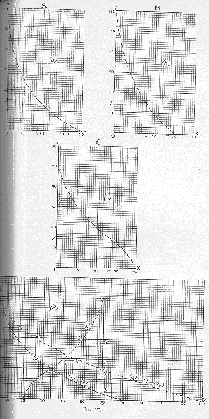 Fig. 20 let us add together in (
d) all the constituent curves except (
c), and instead of adding (
c) as before, let us measure
Ox (the total amount of the stock) along the axis of
X, and taking the point
x as the origin of the curve (
c) let us reverse that curve. The point of intersection will have the same ordinate which we obtained by addition in Fig. 19. This is easily seen from a study of the dotted line, which is constructed, as before, by adding all the curves together. Thus every
mn will equal the corresponding
pq. In the figure,
p3q3 and
m3n3 coincide. Therefore (
Ox being the whole amount of the commodity, and the dotted line being the collective curve)
xn3 is the price that was determined by our former method (Fig. 19). And it coincides with the height of the point of intersection of the sum of (
a) + (
b) with the reversed (
c). Every point on every curve has been taken into equal account in obtaining this result; and it does not matter which curve or curves have been reversed. It is the height of each point that affects the result, not the question whether it has been registered and combined with the others in a curve rising towards the left or one rising towards the right.
What we have now got is an ordinate such that the portions of all the curves which are above it have abscissas that collectively make up the length
Ox, representing the total amount of the commodity.
But this method of intersection can only be applied once. It cannot be applied cumulatively, for it confuses the record while registering the result. Thus if we add (
a) and (
b), and suppose the stock still to be the same, we arrive at
xp as the price which would rule between A and B if C were not in the market; and having C’s curve we can then arrive at the modification in the price effected by C’s entrance into the market either by the method of addition or that of intersection. But suppose we had originally treated (
a) and (
b) by the method of intersection. We should have arrived at the same result as far as they are concerned (
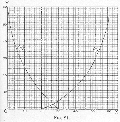 Fig. 21), but we should not now be able to combine it with the data of (
c). Thus it will be seen that the method of addition is the only fundamental one. Intersection is a disguised form of addition, and this very disguise obliterates the record. We shall see the importance of this more clearly as we proceed.
The methods of addition and intersection may both be applied in cases where our data are less complete than we have hitherto supposed; for the process of addition may be regarded as beginning at any point of the collective curve which we like to select. Thus, if we knew, for instance, not how much of the commodity A, B, C, etc., possess collectively, but how much more (or less) than would satisfy them down to the urgency represented, say, by 20, and if we knew the course of the curves in the neighbourhood of the 20 point in each case, we should have all the material necessary for determining the equilibrating price that would satisfy all the consumers, and the ultimate distribution of the aforesaid excess amongst them; but we should not know how distant that point might be from the origin either of the collective or of the individual curves.
We shall enter upon the detailed examination of a case of this kind presently, and it will be seen that it is a perfectly natural one. Our present business is to illustrate it diagrammatically. We are not supposed to have complete knowledge of the curves. We do not know where they start or how they arrive (
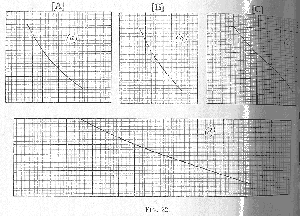 Fig. 22) at the points in (
a), (
b), and (
c), which bring A, B, and C respectively to the margins at which the commodity has a value of 20 for them; nor do we know the total amount of the commodity; but we know how much of it is left when the 20 points in (
a), (
b), (
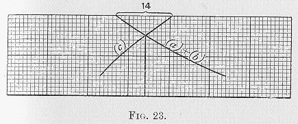
c) have been reached, and we know the course of the curves for some space about these points. Assuming data consistent with those of Figs. 19, etc., let us say that the supply is 14 in excess of that required to bring all the margins to 20. We simply have to add the curves as before, beginning at this point, and we shall obtain a portion of the identical curve (
d) which we had in Figs. 19 and 20, only we shall not know how far off the origin is. We measure off the length 14 from this point, and obtain, as before, 15 as the price. If we preferred the method of intersection we could first add (
a) and (
b), and then reverse (
c), making the space between the highest point of (
a) + (
b) and the highest point of (
c) equal to 14; so that wherever the curves intersect we shall have the collective abscissas of all the curves taken together, above the height of the point of intersection, subtending abscissas to the amount of the stock (
Fig. 23).
It would be a great mistake to suppose that in such a case the portions of the curve and the stock about which we have no information are without influence upon the result. It is because the total amount of stock is what it is and because the curves are what they are that the whole amount of the stock, minus fourteen, is capable of satisfying all the demands down to the ordinate 20. There might, of course, be other combinations of data which would yield the same result, but that would be a coincidence. At any rate the result from which we start is determined by definite data, and our final result is as much determined by those data, of which we only possess the registered results, as by those which are represented by the fragments of the curves and the surplus of the supply which are given us in detail. What ultimately determines the price, then, is the whole amount of the commodity and the character of the individual curves.
We may suppose our information to be given in yet another form. Suppose a whole body of curves (no longer the same body we have represented in Figs. 19, etc.) has been reduced to two (
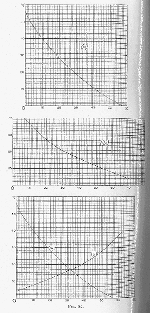 Fig. 24), and we have one of these collective curves given us from the origin onwards (
a). Concerning the other we are told that the total amount of stock (unspecified), if distributed exclusively amongst the consumers represented by this second curve, would satisfy them to the point with the ordinate 4. The course of this curve upward from the point in question towards the origin is given us for a certain distance (
b), but we do not know how far off the origin is. We measure 4 on the ordinate of (
a) at the origin, and then reverse (
b). The point of intersection will give us the price 17. But this again is only a disguised addition of the partial character that we have just examined. We do not know what the quantity of the commodity is, but we know how much it is in excess of any ordinate on curve (
b) which we choose to select, within the limits of our information. Thus we know that it is 63 in excess of the amount required to bring the ordinate of (
b) to 40, 39 in excess of that required to bring it to 20, and so forth. The reversed curve (
b), therefore, will secure that every point is at such a distance from the origin, or highest point of curve (
a), as to comply with the conditions specified in connection with Fig. 23; and the data of the latter figure can be reduced to the form presented in the other with perfect ease. The total amount of the commodity required to bring the ordinate of group (
b) from 40 to 4 is 63. We know from curve (
a) that 10 would be required to bring group (
a) to the same point. Starting then at the points of the two curves with ordinate 40 we have 63 – 10 (=53) as the surplus of the supply; and we can present the two curves from the points of ordinate 40 onwards, with a space of 53 between these two points, and obtain (
Fig. 25) the price by intersection precisely as in Fig. 23. But here, as before, the real process is one of addition. We could of course have started at any other point of (
b) lower than 40, and the corresponding point of (
a), with the same result. In fact our Fig. 25 includes all such alternatives in itself.
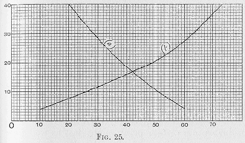
We can now understand the exact meaning of the confirmed habit of presenting the phenomena of the market under the form of a curve of “supply” and a curve of “demand,” the intersection of which determines the price. It is based in the first place on a division (irrelevant as we have seen) between those persons in the market who have, and those who have not, a certain stock of the commodity in question. The curve of the latter is given in its completeness, or, at any rate, the origin is marked and the portion of the curve which is sketched is made to begin at a defined distance from the origin. This is called the curve of demand. The other curve in then inserted as a reversed curve, and a definite ordinate is assumed either for the point at the origin or for a point at a defined distance from the origin; and this is called the supply curve. Now this curve is a curve of reserve prices, which, as we have seen,
*30 is merely another name for the demand curve of those who possess a stock of the commodity; and its reversal is merely a quick way of arriving at the results of addition. But in connection with it information is tacitly given us as to the surplus of the total stock over the amount required in order to gratify the whole market down to some given ordinate. The connection between these two pieces of information is arbitrary; for the vital information as to excess of supply over that required to bring the ordinates to a certain point, might just as well have been given us in connection with the other (so-called “demand”) curve, or partly in connection with one and partly in connection with the other, or without any specified connection with either of them. Thus, if we had not had the two curves given us at all, but only the whole collective curve, without distinction between possessor and non-possessor, and had also been told that the stock was enough to satisfy all claims down to the ordinate of 40 with a surplus of 53, we should have obtained exactly the same result. And if we suppose curve (
a) and curve (
b) alike to be miscellaneous groups, both of them made up of some persons who possess and some who do not possess supplies of the commodity, we shall still have precisely the same results.
But the distinctions which are irrelevant to the determination of the market price and of the quantities ultimately possessed by the individuals constituting the market do affect, as we have seen,
*31 the specific steps by which the price is discovered and the equilibrium reached. It is in the failure to distinguish between the methods by which that price is
discovered, and the ultimate facts by which it is
determined, that the current analysis of the market appears to me to fail. Though the division between buyers and sellers is not absolute (for we have seen
*32 that a man may be a buyer or a seller according to circumstances in the same market, and that the buyer may be a possessor of stock also), yet it is undoubtedly the “higgling” of buyer and seller that discovers the actual price. Hence the seductive character of the current representation, and the insidious character of its concealment of the ultimate nature of the market and market prices.
We will now proceed to the examination in detail of examples of the way in which relevant and irrelevant facts are usually confounded in the analysis of markets and market prices.
In his book on
The Economics of Distribution*33 (pages 11
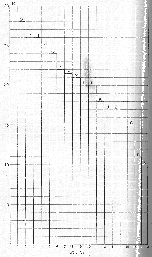
sqq.) Mr. Hobson supposes that in a horse-market there are eight “sellers” (of horses of uniform quality) who have reserve prices running from £10 to £26, and ten “buyers” willing to give prices running from £15 to £30. The details may be thrown into the form of
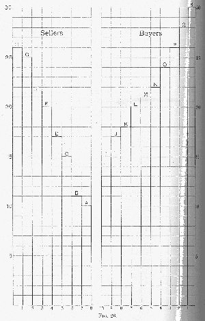 Fig. 26. The figure is necessarily defective, for if H will sell at £26 and P will buy at £26, this involves a difference in the place of a horse upon the scales of preference of H and P, but Mr. Hobson does not tell us how great the difference is. It may be less than a farthing; that is to say, it may be that H would not sell at a farthing less than £26, and P would not buy at a farthing more. But that H would sell at £26 shews that he prefers £26 to the horse, though by never so little; and that P would buy at £26 shews that he prefers the horse to £26. A horse, then, stands on H’s scale at a little below £26, and on P’s at a little above. This is not shewn on our figure; but neither is it necessary for the purposes of our investigation.
Mr. Hobson proceeds to argue that if a price of anything above £21:10s. were set there would be more sellers than buyers, and if anything under £21 were set there would be more buyers than sellers, so that the price would settle somewhere between £21 and £21:10s. Anywhere within this range there would be an equal number of buyers and sellers.
 This is all perfectly true, and it corresponds to our elaborate exposition of the market as a machinery for discovering the ideal equilibrating price.
*34 But if it is given as a statement of the data which determine that price it is quite needlessly complicated and gives us a number of irrelevant facts. If we know nothing at all as to who possess the horses but know the position a horse occupies on the relative scale of each of the persons concerned, we shall have, on
Figure 27, a statement of what prices would rule for any supply of horses from one to eighteen, and shall see that for eight horses it might be anything from £21 to £21:10s.
The relevant facts for determining the price, in the case supposed by Mr. Hobson, are found to be that there are eight horses altogether, and that the places that a horse occupies on the scales alike of A-H and I-R are as stated, and as represented in the diagram. The irrelevant facts are that the eight horses are at present in the possession of A-H, and that I-R are all without horses. When I say that the possession or non-possession of a horse is irrelevant, I mean that it is irrelevant if we know the position of a horse on the scale of preferences of each of the persons concerned. The possession or non-possession of a horse may no doubt affect that position, but so may the man’s health, or the health of his wife, or his age, or the fact that his wife has recently read Mrs. Hayes’s
Horsewoman, or that his daughter has read Xenophon
On Horsemanship, or a thousand other things. There may, in short, be an indefinite number of reasons why the horse occupies just this position on his relative scale, but as long as we know the fact we are indifferent to the causes. Given, then, the relevant facts, you may distribute the items between the groups just as you like. You may arrive at your conclusion by the method of addition or the method of intersection. You may deprive the whole alphabet from A to R of horses altogether, and throw eight horses from some other source upon the market, without reserve price; you may suppose that some in group A-H possess horses and others do not; but you will always bring out the identical result that the market price, virtual or actual, will be somewhere between £21 and £21:10s., and that the ultimate possessors of the horses will be H, G, F, R, Q, P, O, N. Naturally. They are the eight persons on whose scales of preference a horse (whether they have him to begin with or not) stands highest, and there are only eight horses altogether.
If the fundamental method of addition is adopted, it is obvious at once that no hypothesis as to which of the persons brings the horses into the market will in any way affect the result, and, on examination, the same will be found true if we adopt the method of intersection. On Mr. Hobson’s supposition, group I-R possess no horses, and group A-H possess eight. We know, then, that as there are eight horses altogether, we must so arrange the curves that between the highest of one group, R, and the highest of the other group, H (both included), there shall be eight units, so that whatever the point of intersection may be there shall be eight and only eight letters above it. This will give us
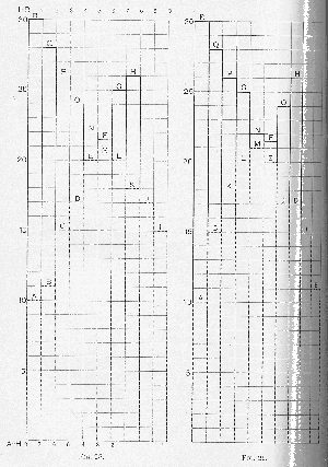 Fig. 28,*35 which will bring out the same ultimate possessors of horses and the same prices as we had in Fig. 27. But if we suppose that the eight horses were originally possessed by A, C, F, H, K, L, M, O, and that B, D, E, G, I, J, N, P, Q, R were without them, and proceed by intersection to determine the price and the ultimate possessors, we must again see to it that between R and H (both included) there are eight units, and again we shall obtain identical results (
Fig. 29). But this rearrangement of the individuals is really superfluous. We may suppose the down and up sloping series in Fig. 28 each to include possessors and non-possessors, according to the data of Fig. 27. This will in no way affect the result; nor is it necessary to have any information on the subject in order to split up the data of Fig. 27 in any way we like and place the two groups cross-wise, with the interval between their highest members determined by the datum as to the total number of horses.
It will be noted that Mr. Hobson gives us the whole of the facts. Mr. Marshall (
Principles of Economics, ed. 3, page 410) has a parallel example in which he only gives some of them. He supposes, in a corn-market, that at 37s. a quarter there will be “sellers” of 1000 quarters of wheat and “buyers” of 600; at 36s. “sellers” of 700 and “buyers” of 700; at 35s. “sellers” of 500 and “buyers” of 900.
The facts given us may be tabulated thus:—
| A | B | ||
| Sellers will sell— | Buyers will buy— | ||
| 1000 | at 37s. | 600 | at 37s. |
| 700 (keeping 300) | at 36s. | 700 | at 36s. |
| 500 (keeping 500) | at 35s. | 900 | at 35s. |
Therefore (subtracting from the B figures the 600 required to bring the B’s to the 37s. point) we find that when all are satisfied down to the point of 37s., it will take—
| A | B |
| 300 more to satisfy the A’s to the point of 36s. | 100 more to satisfy the B’s to 36s. |
| 500 more to satisfy the A’s to the point of 35s. | 300 more to satisfy the B’s to 35s. |
It appears, then, that in the market altogether there are 1000 quarters more than would satisfy the group A, called “sellers,” down to 37s. (for they have 1000 quarters that they value at less than 37s., or they would not sell them at that price). It would take 300 of these to satisfy them down to the point of 36s. (for we are told that at 36s. they would hold back 300), and 200 more to satisfy them down to 35s. What we know of the curve of the group called “sellers” is therefore represented on
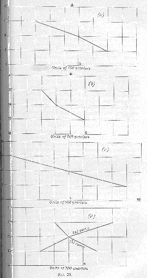 Fig. 30 (
a). As to the group B, called “buyers,” we do not know to what point they are already satisfied,
i.e. we do not know at what price they would begin to buy, but we know that 600 quarters (or 600 more than they already have) would bring them to the point 37s., and then another 100 would bring them to 36s., and another 200 yet to 35s. What we know of their curve, then, from the 37s. point onwards is represented on Fig. 30 (
b). In neither case do we know how far from the origins the curves start.
Let us add the two curves, starting at the points with the ordinate 37s. Fig. 30 (
c) gives us the result. Now we know that after all parties are satisfied to the point of 37s. there are 400 quarters left; and these will satisfy all parties to the point of 36s. Or we might adopt the method of intersection, placing 400 quarters between the 37s. points of the two curves. The result, of course, will be the same (
d). Both (
c) and (
d) can be constructed and read without reference to the initial distribution of the corn. If all the corn had originally been in the possession of the group A, or if half of it had been in A’s possession and half in B’s, or whatever the proportion had been, so long as the curves of significance remained the same, and the excess over the amount required to bring them all to the point 37s. remained 400, we should always have the same result. The course of the curves, then, and the amount of the excess, constitute our relevant information—relevant, that is, to the determination of the market price and the ultimate distribution of the excess. The irrelevant information is that the corn is now in the possession of group A.
A psychological objection may here be raised. It may be said that it is impossible that the curve of preference should be conceived irrespective of the possession or non-possession of the commodity. In the case of the horse-market it may be admitted that every man has a more or less determined relative estimate of the significance of a horse, and that we need not inquire how he came to form it. But in the case of the wheat we are asked to suppose that each man has a scale on which successive quarters of wheat are continuously registered with continuously declining significance. Now it may very well be that the man who comes into the market with the intention and hope of selling may buy when he becomes better informed of the facts, or
vice versa, yet some mental friction would have to be overcome, so that the curve would not decline regularly, but would break at certain points determined by the amount of corn the man possessed. The answer is that this may be, though it need not be, the case; but that in a large market such individual considerations will counteract each other, and the whole body of persons conducting the business will present a sensibly continuous curve.
The final outcome of these investigations is that the diagrammatic method of taking a buyers’ curve and a sellers’ curve and shewing by their intersection what the market price will be is perfectly legitimate if properly understood, but that if it is supposed to represent the ultimate facts which determine the price, it embodies and emphasises irrelevant matter. If it is supposed that the two curves are different in kind and represent two principles, that they could not equally well be represented as a single curve, or that the transference of any constituent elements from one to the other would affect the result, or that either curve might not contain the register of both buyers’ and sellers’ preferences, then the method is misleading and mischievous. In the higgling of the market the price
emerges as the result of the play of a conflict between buyers and sellers as such, which is not relevant to the ultimate facts and forces which
constitute that price. The method of intersection is, in fact, a mere disguise of the method of addition, and it might ignore the distinction between buyer and seller without affecting the result, as far as price and ultimate distribution are concerned. If adopted to shew the amount of business done under given conditions, the distinction between buyers and sellers and the intersection of their curves is a legitimate method; if adopted to shew the ultimate considerations that determine the market price, it is, to say the least of it, seriously misleading.
Our main conclusions are nothing new. They merely restate the results of the analysis of markets entered upon in Book I. Chapter VI. Given the total supply of the commodity, the market price that any single customer finds established is determined in the main by the demands of all the other purchasers, but in some degree by his own. If his demand is, in bulk, a very small portion of the whole, then its effect on the price will be correspondingly small, that is to say, the total curve will decline so slowly that the addition or withdrawal of an amount of the commodity sufficient to carry this one purchaser from his initial to his final increments will not perceptibly raise its ordinate. And therefore in dealing with any one individual separately we may assume the market price as already fixed by all the other individuals, and may then simply measure it off on the axis of
Y of the particular curve we are examining, and may draw a parallel to the axis of
X through that point. The abscissa of the point at which this parallel cuts the curve will measure the amount that this particular purchaser will take. We may put it in this way: the amount of any commodity which will flow, in obedience to the economic forces, to the satisfaction of any one consumer’s wants will be determined by his curve of preferences, by the similar curves of all the other claimants, and by the total amount of the commodity. This is the general law of distribution.
If we go on to ask what determines the quantity of the commodity, we find ourselves dealing once more with the identical problem that we have just solved. The flow of the productive forces into this or that industry is determined on exactly the same principles as the flow of the stock of any single commodity to the different consumers. To breed horses you need land, buildings, corn, apparatus of many kinds, and trained human faculty. In supplying horses, therefore, you demand all these things. To raise corn you need land, buildings, ploughs, waggons, gates, ships, machinery, and human faculty. In supplying corn, therefore, you demand these things. And so with all other commodities. Thus the supply of any commodity is itself a demand upon other commodities and services, and if we separate out the demand, say, for woodwork implied in the supply of each of the commodities into which it enters, we shall be doing just the same thing that we did when we separated out the demand for potatoes from all the individual budgets of the persons that composed the market. Here, as there, the share that each one gets is determined by the curve representing the urgency of the want it satisfies, by the similar curves of the other industries, and by the total available resources of the community. Thus the supply of any commodity is regulated by the combination of productive factors needed for its production and the rival claims of other commodities for the factors of this combination. Ultimately, then, we have at one end the undifferentiated and unmanipulated forces and materials of nature, the faculties (trained and untrained) of man, and the various modifications of the former by the latter, which exist at the moment. This constitutes the total available stock. And at the other end are the tastes and resources of each individual. The amount of the supply, at any moment, of this or that commodity (in its final and united form, or in any of its intermediate states or constituent elements) is determined by the attempts of the commercial community to gauge and anticipate individual wants and to regulate the flow and the combinations of the ultimate sources of supply in accordance with them.
We have seen that all the different items of the ultimate sources of supply, and all the existing products, can, at any given moment, be expressed in a common unit. Therefore, in considering any single industry, we have first to determine what unit we will take to measure amounts of the productive agents. We might take, for instance, the amount that would exchange for an ounce of gold, or a ton of pig-iron, or a quarter of wheat of given quality, or any combination of these or other articles we choose to select. This will be our arbitrary unit-of-products-and-factors-of-production, and as we are now applying it exclusively as a measure of factors of production we will call it the unit-factor of production. The unit of the special product we will take as that amount of it which the unit-factor of production can produce. What will the unit on the axis of
Y be? It will represent the general command of articles in the circle of exchange which corresponds to the ounce of gold, ton of pig-iron, or what not, that we have taken to measure our unit-factor of production. We may think of it in terms of money. It may be a pound’s worth or a shilling’s worth of anything that is in the circle of exchange, including the factors of production themselves. The curve, then, will indicate the place on the communal scale of preferences of each successive unit of the commodity; and the flow of productive forces into that industry will be regulated exactly as the flow of fish or carrots to this or that purchaser’s larder is regulated. It will bring it down to the (objective) level determined by its marginal significance elsewhere. If the total amount of the resources of society which will in any case be deflected to this particular industry is an infinitesimal portion of the whole, we may take this margin as independently fixed. The curve (
Fig. 31) gives us the rate at which the unit-factor of production will satisfy human wants (measured objectively) in this industry at any margin.
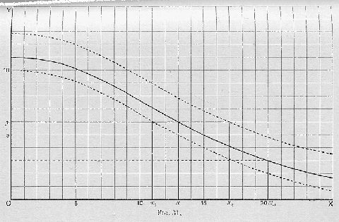
At what rate (measured by the same standard) will it satisfy human wants in other marginal applications? Whatever that rate may be it can be represented by a line. Measure off that line on the axis of
Y, draw through the point thus determined a parallel to the axis of
X, and the abscissa of its point of intersection with the curve will determine the flow of the productive resources to this industry, and the corresponding amount of the product. The curvilinear space above this line will represent (objectively) the satisfaction which the creation or destruction of this particular industry would add or subtract from the community. Its revenues of enjoyment (or at least of anticipated or estimated satisfaction) will be increased to that extent by the existence of this industry. It follows, of course, that whereas the communal curves of demand for, say, a certain kind of timber in the furnishing, the building, the shipping trades, and so forth, can be added, under the conditions laid down on pages 494
sq., the communal curves for different commodities (houses, ships, race-horses, diamonds, books, fruit, music, etc.) cannot be added, since each such curve assumes that all other conditions remain the same, and to travel along any one of them constitutes a change of the conditions for some or all of the others.
If the demand (estimated significance) for a commodity increases, as represented by the upper dotted line in Fig. 31, the product will be increased from
Ox to
Ox1. If it declines, as in the lower dotted line, the industry will shrink to
Ox2. If, while the demand remains the same, some invention is made which doubles the quantity of the commodity which could be produced by the unit-factor of production, or, which is the same thing, halves the amount of the productive forces required to produce the units we have hitherto registered along
Ox, the dotted line parallel to the axis of
X will indicate the quantity which will be produced. We might equally well represent this latter change by retaining the length
Oy unchanged and doubling the height of the ordinate at every point, because the factors that would give the value
Oy in other industries will now be producing the units of our product, and therefore the anticipated satisfactions they yield, at double the previous rate. The unit of
Ox, therefore, will represent twice as much of the commodity, measured in its own proper unit, as before (
Fig. 32).
 We have now to note that any very extensive departure from the existing state of things might affect the whole constitution of the unit on which we are working, for it might disturb the marginal relations between different kinds of human effort and different products or gifts of nature. And, as the value of anything can only be expressed objectively in terms of something else, changes or discoveries that affect the general fertility of human effort, and the significance of natural products and agents, cannot be recorded by any consistent objective method. Further, the diagrammatic illustrations which we have been using can only be regarded as applicable to cases in which we are examining a very small part of the whole field, so that we may consider the general conditions as stable. An attempt to draw up the whole scale of significance of any one of the main factors of production, carried back to the origin, would of course be quite futile. It would be impossible to imagine the origin at all nearly approached without such a disturbance in other conditions as would deprive our units of all continuous significance.
One other point of theoretical interest remains for investigation here. We have seen
*36 that the creation of the supply of undifferentiated human capacity is to be regarded in the main as itself constituting a branch of expenditure or “consumption.” It is determined, at any moment, by the scale of relative significance of this particular form of expenditure, “consumption,” or expression of impulse, which has ruled in the past. But the total capacity-for-effort that exists is not employed “economically.” What determines the amount that is devoted to the production of things that enter, or might enter, into the circle of exchange? Here, as in previous instances, we must begin with individual curves. Writers who have paid attention to the subject have usually regarded the output of human effort (spoken of under the rather dangerous abbreviation of “labour”) as limited by its irksomeness, and have represented its significance (at least after a certain point) as a negative quantity.
We will begin with Robinson Crusoe. Along the axis of
X (
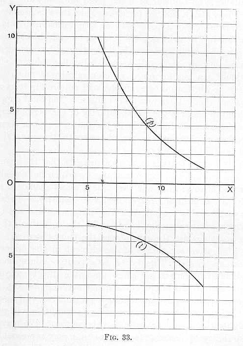 Fig. 33) we measure units of effort. The proper basis for such a unit would be foot-pounds if we were considering mere muscular effort, but it will be convenient to take an hour’s work as our unit, including all physical and mental effort, and ignoring the fact that during different portions of the day, and so forth, the actual output of effort made per hour, measured by any objective standard, will vary. The
p curve will now represent the marginal significance to Crusoe of the result of successive unit-outputs of effort, and the
l curve will represent the marginal irksomeness of the output of effort itself. The unit on the axis of
Y is essentially psychic, and we may for the present read the figure as meaning simply that at the margin of six hours’ work per day the value of the product compensates threefold the irksomeness of the effort; that is to say, Crusoe would make the effort even if its results accrued at only a trifle above one-third the rate at which they actually accrue. Thus the balance is favourable up to 9 on the axis of
X; after that it would be unfavourable, and therefore the output of effort is carried to that point and no further.
Leaving the island and returning to civilisation, we take the remuneration of each man’s effort per hour as a datum, fixed by the general laws of the market, and, still reading the curve psychologically, we find that at the margin of six hours a day the individual whose curve we are examining estimates the advantage of the increased supplies of all commodities and services in the circle of exchange as threefold compensation for the irksomeness of the work that secures them. And the advantage is on the side of doing more work for wages up to nine hours a day, but no further. This, then, is the amount of labour he chooses to supply on the terms which it will command in the market. Well, then, he sells his time with a system of reserved prices, which constitutes his own demand for it; just as the stall-keeper sells her plums.
*37 Each individual can get for his work economically as much as his doing it is worth to others, and he will require for it as much as his not doing it is worth to himself. The total supply of any kind of effort is the whole capacity of the persons capable of making it, and this supply is distributed between economic and other applications in accordance with the general laws we have studied so fully.
This way of putting it at once suggests that the man who sells his labour is selling something for which he himself has a demand of some kind, and that this demand should be represented as a positive, not a negative quantity. Reflection fully justifies this suggestion. The irksomeness of the labour by which we earn money is not really the only thing that we have to set against the advantages the money secures. It is only a negative expression of one element in the desirability of rest or leisure.
 This latter is a positive conception, and it includes all output of effort upon the direct securing of things not in the circle of exchange, as well as rest. Our previous studies
*38 of the relations of positive and negative satisfactions and their diagrammatic representation will remove all difficulties from our path in this matter. We may treat “desirability of leisure” as positive, and may represent the
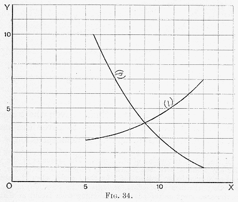
l curve with positive ordinates, as in
Fig. 34. We shall then get the same point as before, viz. 9, by intersection, and shall see that the whole diagram is no more than another disguise of the process of addition of curves.
We may read the
l curve, whether in Fig. 33 or in Fig. 34, thus:—We have no information as to the total of exchangeable commodities which the man could conceivably secure to himself by his extreme output of effort, reducing his leisure to the minimum requirements of rest and nutrition which would enable him to continue at the same level. But we know that if he had already reserved as much leisure as would reduce its marginal significance to 7, he would still have thirteen hours a day, to distribute between the further gratification of his desire for more leisure and the total gratification of his desire for things in the circle of exchange. The
p curve shews us that it will take seven of those thirteen hours to bring his desire for things in the circle of exchange down to the point of 7. That is to say, the marginal value of leisure, when eleven hours have been reserved for it, and of the reward of labour, when seven hours have been devoted to it, stand alike at 7. There are six hours more to be distributed between them. Add the curves together from this point, reversing
l (
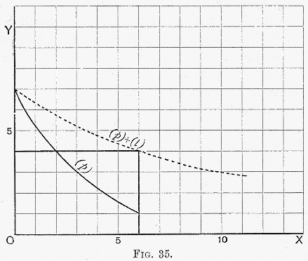 Fig. 35), and we shall obtain our former result as to the point to which both sets of desires will be gratified. Two more hours will be devoted to work, making nine hours altogether, and four more to leisure, making fifteen hours altogether.
*39
For obvious reasons we have not carried our curves back to the origin. The assumption that “other things are equal” would be patently absurd at any great distance from the actual point of equilibrium. Even the range that we have actually allowed our curves to cover can only be justified by considerations of facility of demonstration.
sq.
sqq.
sqq.
sqq.
sqq.
sq.
sqq.
sqq.
l curve we have assumed a stability in our psychic unit on the axis of
Y that was not granted in our first construction of the figure. The ordinates of the
p and
l curves for any abscissa were determined with reference to each other, at that point, and consequently our ordinate of 7 for the
l curve, when the abscissa is 13, means that irksomeness of effort (or desire for its cessation) at that point is seven times as great as the advantage accruing from labour at that point. It does not follow that it is just equal to the advantage accruing at the abscissa 7, unless we can be sure that the psychic value of the unit remains stable for
p throughout its course; and we have seen (pages 469
sqq.) the extreme difficulty of securing even a fair approximation to such stability in far simpler cases than this. If we retain the form of the
p curve, and reversing the
l curve relate each ordinate to the now corresponding ordinate of
p, we may get a different form of the curve, representing the same relations and the same psychic values. But the point at which the two ordinates are equal to each other must obviously be the same.
