The Theory of Interest
By Irving Fisher
THE tremendous expansion of credit during and since the World War to finance military operations as well as post-war reparations, reconstruction, and the rebuilding of industry and trade has brought the problems of capitalism and the nature and origin of interest home afresh to the minds of business men as well as to economists. This book is addressed, therefore, to financial and industrial leaders, as well as to professors and students of economics.Inflation during and since the War caused prices to soar and real interest rates to sag in Germany and other nations far below zero thus impoverishing millions of investors. In all countries gilt-edge securities with fixed return became highly speculative, because of the effect of monetary fluctuations on real interest rates. After the War the impatience of whole peoples to anticipate future income by borrowing to spend, coupled with the opportunity to get large returns from investments, raised interest rates and kept them high. Increased national income has made the United States a lender nation. At home, real incomes have grown amazingly because of the new scientific, industrial, and agricultural revolutions. Interest rates have declined somewhat since 1920, but are still high because the returns upon investments remain high. Impatience to spend has been exemplified by the organization of consumers’ credit in the form of finance companies specially organized to accommodate and stimulate installment selling and to standardize and stabilize consumption…. [From the Preface]
First Pub. Date
1930
Publisher
New York: The Macmillan Co.
Pub. Date
1930
Comments
1st edition.
Copyright
The text of this edition is in the public domain.
- Dedication
- Errata
- Preface
- Suggestions to Readers
- Part I, Chapter 1
- Part I, Chapter 2
- Part I, Chapter 3
- Part II, Chapter 4
- Part II, Chapter 5
- Part II, Chapter 6
- Part II, Chapter 7
- Part II, Chapter 8
- Part II, Chapter 9
- Part III, Chapter 10
- Part III, Chapter 11
- Part III, Chapter 12
- Part III, Chapter 13
- Part III, Chapter 14
- Part IV, Chapter 15
- Part IV, Chapter 16
- Part IV, Chapter 17
- Part IV, Chapter 18
- Part IV, Chapter 19
- Part IV, Chapter 20
- Part IV, Chapter 21
- Appendix to Chapter I
- Appendix to Chapter X
- Appendix to Chapter XII
- Appendix to Chapter XIII
- Appendix to Chapter XIX
- Appendix to Chapter XX
- Appendix to Chapter XX
§1. Introduction
PART III, CHAPTER X
FIRST APPROXIMATION IN GEOMETRIC TERMS
PART III. THE THEORY IN MATHEMATICS
WE found in Chapter V that, if the degree of any given individual’s impatience depended solely on his income stream, and if that stream could not be modified through the loan market or otherwise, his impatience could not be modified either. In such a world of hermits, each person would have his own individual rate of time preference, the various individual rates ranging from several thousand per cent per annum down to zero, or below. In such a world, since there would be no loans, there would be no market rate of interest.
But we also perceived that, as soon as our hermits are allowed to swap income streams, one man exchanging some of this year’s income for some future income of another, then these myriad rates of time preference or impatience tend to come together toward a common rate, and, on the assumption that no risk attends these transactions, a uniform market rate of interest would actually be reached. In such a perfect loan market the degree of impatience of each person would become equal to that of every other person and to the rate of interest.
§2. The Map of This Year’s and Next Year’s Income
Expressing the problem with the aid of the graphic method, the determination of the rate of interest may
be reduced to a simple problem of geometry, just as the problem of price may be shown by supply and demand curves.
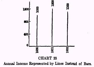
To depict adequately the elements of the interest problem, however, a new kind of chart is required. Our first task is to see the relation of this new kind of chart to those hitherto used in this book. First, then, let us recur to Charts 1, 2, and 3, in Chapter I, which picture a person’s income stream over a period of years. This sort of chart consists of a row of vertical bars representing the real income, as measured by the cost of living in successive periods—days, months, or years. To prevent confusion, let us, for our present graphic purpose, shrink these vertical bars into mere vertical lines, without breadth. Then, each year’s income may be pictured as if it were all concentrated at a point of time, say in the middle of the month or year concerned. Since the rate of interest is usually expressed in
per annum terms, it will simplify the discussion if these lines are drawn, as in Chart 23, disregarding all time units other than years. To make our
picture still more concrete, specific figures may be attached to specific years, the person’s income for 1930 being set at $1000, that for 1931 at $1200, and so on.
We are now ready to pass to the new and radically different method of representing the real income stream. In the chart just described, horizontal distance measures time, while vertical distance measures amount or size. The reader is now asked to shake off these conceptions. Moreover, throughout Chapters X and XI, he must be on his guard against their unconscious return. In the new charts there is no time scale; time is not measured at all; both axes measure amount of income. The horizontal axis represents the first year’s income, the vertical, the second year’s income. Thus the point
P1 in Chart 24, through its latitude and longitude, stands in a sense for both years’ incomes combined. It represents what may be called a given individual’s income combination, income stream, income position, or income situation for the given pair of years. On Chart 24 may be shown a complete map of all possible income combinations, or income positions, so far as two years, or periods of time, are concerned. To represent the third year, so easily shown in Chart 23 under the old method, we should need in this new method a third dimension. The chart would then cease to be a chart and become a three dimensional model.
*1
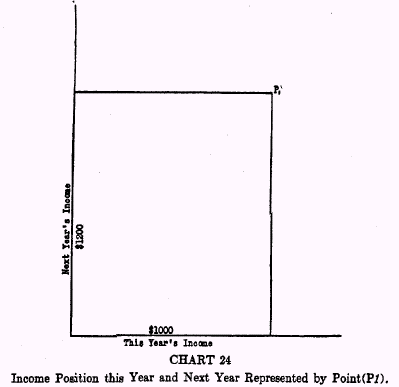
If on the map for two years, we were to draw a straight line from the origin toward the “northeast”, midway between the two axes, every point on it would have its longitude and latitude equal, that is, would represent different
income situations in which the incomes of two years were equal. A poor man—poor in both years—would be situated near the origin, and a rich man far from the origin. A man who has less income this year than he expects to get next year would be situated above this midway line, his latitude (meaning next year’s income) being more than his longitude (meaning this year’s). If we move his position sufficiently to the left, so as to reduce his longitude (this year’s income), he will be like a man stranded on a polar expedition—with rations run short, though he might be assured by radio of plentiful
supplies next year. On the other hand, a man who is more abundantly provided with income this year than he expects to be next year would be situated
below the midway line, his longitude being greater than his latitude.
In this way, within the northeast quadrant (the only one shown in the charts) we can, by fixing the point
P at all possible positions, represent all possible combinations of this year’s and next year’s income.
§3. The Market Line
Assuming that the individual’s incomes for all other years remain unchanged, we shall now study the effects, for this one man, of changing the income amounts of the two years pictured. These changes are assumed to be caused wholly by trading some of his income of one year for some of another man’s income for the other year. Except for such trading, his income situation is supposed to be fixed. He has, let us suppose, a rigid allowance of $1000 for this year and $1200 for next year with no opportunity to change these figures except by swapping some of one year’s income for some of another’s.
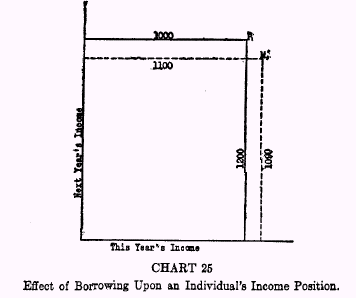
Suppose, for instance, that at a rate of interest of 10 per cent the individual borrows $100 in 1930 in return for $110 which he is to pay back in 1931. In Chart 23, such changes would be represented by lengthening the 1930 vertical line from $1000 to $1100 and by shrinking the 1931 vertical line from $1200, not to $1100 but to $1090. In Chart 25 these changes are represented by shifting the income position from
P1, the originally fixed income position, to
M1, whose longitude is $100 more and latitude $110 less.
If, as shown in Chart 26, the individual borrows a second $100, promising to repay $110, his income position
shifts again, this time from
M1‘ to
M1”, that is, from this-year-1100-and-next-year-1090 to this-year-1200-and-next-year-980. Borrowing a third $100 would bring him to
M1”’, (this-year-1300-and-next-year-870). Every additional borrowing of $100 adds $100 to this year’s income and subtracts $110 from next year’s income. Chart 26 pictures these successive changes as a “staircase” of which each “tread” is $100 and each “riser” is $110. The stairs are steep. So long as there exists a rate of interest their descent is
necessarily always faster than 45 degrees—that is, future income decreases faster than present income increases; the riser is more than 100 per cent of the tread—more by the rate of interest.
*2
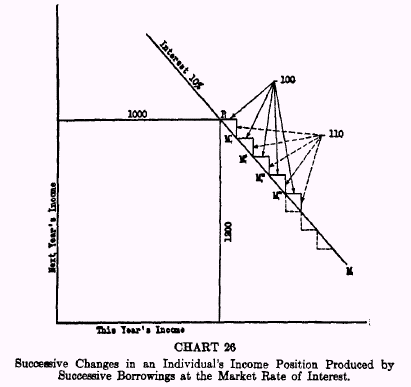
If the rate of interest were zero, each $100 borrowed would require only $100 to be returned next year. The riser would equal the tread; the Market line would make an angle of 45° with the axis, and its slope would equal unity, or, in other words, 100 per cent. Thus in this new method of charting, a given rate of interest is represented by the algebraic difference between the slope of the given Market line, and the 100 per cent slope of the 45° zero interest line.
Evidently the line
P1M1 is a straight line. It may be called the Market line, Loan line, or Rate of Interest line, and, if prolonged, will contain all the positions to which this particular individual (who may be called Individual
1)
can shift his income position by borrowing or lending.
If, starting at
P1, he shifts
down this straight staircase (southeast) he is a
borrower or a
seller of next year’s income, because he is adding to this year’s income and subtracting from next year’s. If, instead, he shifts
up the staircase (northwest) he is a
lender or
buyer of next year’s income, subtracting from this year’s income and adding to next.
§4. The Willingness Line
So far we have used the new type of chart only to show how the individual
can move—change his income situation. The next question is: in which one of the two directions on the Market line
will he actually move? The answer depends on his degree of impatience compared with the market rate of interest. We have seen how the market rate of interest is represented graphically by the slope, relatively to 45°, of the Market line in Chart 26. We are now ready to make a similar graphic representation of the individual’s rate of time preference or impatience. This is expressed by a series of curved lines showing on what terms, at any income position (such as
P1), the individual would be
willing to lend or borrow, say $100. What one is
willing to do and what he
can do are two quite different things. The Market line of Chart 26 shows what he
can do, while the Willingness lines, now to be described, will show what he would be
willing to do.
Individual
1‘s impatience is such that he would be
willing, if necessary, as shown in Chart 27, to borrow his first $100 at 30 per cent, considerably above the market rate, 10 per cent. That is, he would be willing to sacrifice $130 out of next year’s income in order to add $100 to this year’s income. To get a second $100 this year, he would not be willing to pay quite so much, but only, say, $120. A third $100 would be worth to him only $110; a fourth still less, and so on. These willingness points make a
curved staircase, the steps being from
P1 to
W1‘, from
W1‘ to
W1”, and so on, in which each tread is taken to be $100, but the risers are decreasing as the borrower steps down southeasterly, being successively 130, 120, 110. The
Willingness line,
P1W1IV, is not a straight line like
P1M1 in Chart 26, but a curved line. The steepness of each step, or ratio of risers to tread, or slope of the curves shows the degree of impatience at that particular step.
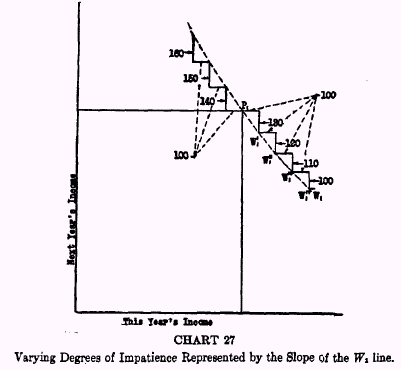
The Willingness line through
P1 extends, of course, in both directions. It shows not only on what terms Individual
1 would be willing to borrow, but also on what terms he would be willing to lend. At point
P1, he is willing to lend the first $100 at 40 per cent, a second, at 50 per cent, and so on. Everyone theoretically is ready either to borrow or to lend according to the terms. Individual
1 is here represented as barely willing at
P1 either to borrow $100 at 30 per cent, or to
lend $100 at 40 per cent. In short, he would be
willing to substitute the combination represented by any given point on his Willingness line for the combination represented by any other point on the same line.
All points on that line are, by hypothesis, equally desirable to Individual
1. Each segment of the Willingness line, by the divergence of its slope from 100 per cent, shows the degree of impatience at the particular income position there represented.
Consequently,
P1W1 might be called an Impatience line quite as well as a Willingness line
*3 for Individual
1. There would be another Willingness line, or
W line, for any other individual. The
W lines thus differ from the Market, or
M, lines which are common to everybody in the market.
§5. The Two Lines Compared
The
M line of Chart 26 and the
W line of Chart 27 are brought together in Chart 28. From
P1 we have a pair of
lines, one (
M1) showing by its divergence from the 45° slope the rate which Individual
1 can get, as a borrower, and the other (
W1) showing by its slope the rate at which he is
willing to borrow. Evidently if he is willing to pay 30 per cent for a $100 loan when he can get it at 10 per cent, he will borrow. Evidently also he will continue to borrow as long as his willingness rate, i.e., his rate of time preference or impatience, is greater than the rate of interest, in other words as long as, at each stage, the Willingness line is steeper than the Market line.
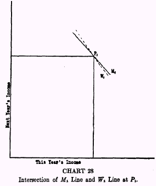
All that has been done so far is to describe the income map, and to place on it a point
P1 to represent the assumed
fixed income situation of Individual
1, and to draw through this point
P1 two lines, one a straight line, the Market line, showing the direction in which Individual
1 can move away from
P1, and the other a curved line, the Willingness line, showing the direction in which he is
willing to move. He is
willing to borrow a first $100 at 30 per cent, or lend a first $100 at 40 per cent, but
can do either at 10 per cent.
§6. The Whole Family of Market Lines
But before we make use of the contrast between the
M and
W lines to follow the individual as he moves his income position from
P1 either northwest as a lender or southeast as a borrower, we must first complete our pictures of the two kinds of lines. Thus far only one line of each of the two kinds has been drawn. These are the only lines applicable to the given income position
P1. But for every other income position in which we may place Individual
1, the Market line would encounter a different Willingness line.
In the same way, we could picture a series of pairs of Market and Willingness lines for any other individual, such an Individual
2, depicted in Chart 29. In this case, Individual
2 is represented at one position to be willing to
lend at 2 per cent but to be able to do so at 10 per cent, the market rate; we have then the Market line
P2M2 and the Willingness line
P2W2. In the same way, we could draw
P3M3 and
P3M3, for a third individual and so on.
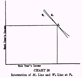
Under our assumption of a perfect market, all the Market lines
P1M1,
P2M2,
P3M3, etc., are parallel to each other, their common divergence from a 100 per cent slope representing the one universal market rate of interest, here supposed to be 10 per cent.
*4 Since the Market lines are thus parallel, they are really impersonal or independent of particular individuals, and we may consequently picture the whole map (Chart 30), as covered with straight and parallel Market lines, like the conventional picture of a rainstorm, each line being slightly steeper than 45°, and its divergence therefrom indicating a rate of interest.
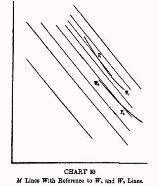
§7. Many Families of Willingness Lines
The Willingness lines, on the other hand, are personal, or individual. The particular slope in each case is, of course, dependent on the particular income position
P1. A given Individual
1 is concerned with only one Willingness line at a time, out of his whole “family” of lines—the one line which passes through his actual income position at
P1. By comparing his Willingness line at that particular point with the Market line, we have a graphic picture of the motives which decide whether he will borrow or lend.
There always exists for him, potentially, other Willingness lines, passing not through his actual income position
P1, but through any other income position at which he could be imagined to be. These curves represent the various rates at which Individual
1 would be willing to borrow or lend if his income position were varied. Thus
the number of Willingness lines for any one Individual is infinite, and every other individual will have his own family of lines.
We conceive, then, of a map for Individual
1 alone, covered with a family of such Willingness lines infinite in number, arranged so as to vary gradually from each to the next, like the lines of elevation on a geographic contour map of a mountain.
*5
While Individual
1 finds all points on any one Willingness line of
equal desirability or “wantability,” he would
rather have his income position on lines more to the “northeast,” or farther from the origin. Each Willingness line might be labelled with a number representing specifically the total desirability or “wantability” pertaining to each and all of the income positions on it. It is the locus or assemblage of these points (combinations of income for the two years) equally desirable in the estimation of Individual
1. A greater aggregate income in the two years may be offset in respect to the resulting total desirability by a less convenient distribution between the two years and
vice versa.*6
But we are not yet interested in such differences of level or total desirability between the Willingness lines. We are here interested only in the
directions of the Willingness lines at different points, representing the different
degrees of impatience pertaining to different income situations. These directions, or divergences from the 45° line, picture to us how the individual would be willing to borrow or lend under all possible income circumstances.
§8. A Typical Family of Willingness Lines
While we cannot, of course, tell exactly how any human being would act if far from the income situation in which he is actually placed, yet we know what in a way would be characteristic of him. Chart 31 is believed to represent roughly a family of Willingness lines typical of most human beings. It is best analyzed by following the dotted straight line
SS‘ running northeast, midway between the axes and therefore comprising points which represent, in each case, equal incomes in both years.
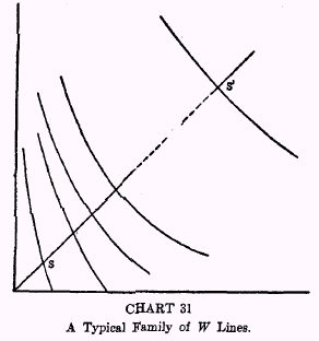
Four characteristic properties may be noted:
(1) At
S, taken to represent a point near the minimum of subsistence—the income situation, say, of a polar explorer who is marooned and hopeless—the Willingness line is nearly vertical. In this income position of extreme need a person would scarcely be willing to lend at all, for to give up one iota of this year’s income in exchange for any amount promised for next year would mean too great a privation in the present. On the contrary, in order to get an added dollar today to help keep body and soul together this year, he would be willing to give not only 10 per cent or 25 per cent but perhaps as much as 100 per cent, or 1000 per cent, or
every dollar of next year’s income even though next year is no more promising than this year.
(2) At
S‘, taken to represent an exceedingly large income—say $1,000,000 for each of the two years—the Willingness line is nearly at right angles to the
SS‘ line; that is, nearly at 45° to the two axes, for with such a large income the two years would seem almost on even terms. Presumably one with this income would not be willing, in order to get $1000 more income this year, to give up much over $1000 out of next year’s income.
(3) As one passes between the two income situations above mentioned, from
S to
S‘, his rate of time preference will gradually decrease—from nearly infinity at
S down nearly to zero at
S‘, that is, the larger the income, other things remaining the same, the smaller the degree of impatience.
(4) Any one Willingness line grows steeper as it proceeds upward and leftward, changing from a nearly horizontal direction at its lower right end to a nearly vertical direction at the opposite end.
§9. Time Preference May be Negative
If these specifications are correct, some, at least, of this family of Willingness curves, especially those far distant from the origin, and low down—that is, representing small
future and large
present income—will have an inclination
less steep than 45° to the horizontal axis and a slope less than 100 per cent. At such income positions the rate of time preference would be negative. It is sometimes said that it is a fundamental attribute of human nature to prefer a dinner or a dollar this year to a dinner or a dollar next year, but this statement is evidently too narrow. Unconsciously it confines our view to regions of the income map where present income is relatively small or future income relatively large. For a starving man it is notably true, that is, the Willingness lines that lie in
the left part of the map are far steeper than 45°. Of a man expecting large future income it is also true; that is, the Willingness lines
toward the top of the map are also very steep.
But if we turn our attention in the opposite direction—to the right, or downward, or both—we find regions on the map in which, if the foregoing description is correct, the curves flatten out and incline less than 45°; the man’s income situation is such that he might even be willing to lend for nothing, or even less than nothing, simply because he would, in such a case, be so surfeited with this year’s income and so short, prospectively, of next year’s income that he would be thankful to get rid of some of this year’s superfluity, for the sake of adding even a trifle to next year’s meager real income. His situation would be like a Robinson Crusoe on a barren island, well supplied, but with foods that could serve him only this year. Such
situations are rare in practice, but they are certainly imaginable and sometimes even occur. In such situations a man would be willing to save for the future without any incentive in the form of interest. But this takes us beyond our present point; for here we are concerned only with the Willingness lines, not with the Market lines.
§10. The Personal and Impersonal Influences on Impatience
By the aid of this map we can see, anew, and more clearly, that a man’s actual degree of impatience depends on two circumstances:
(1) It depends on his “personal equation,” the whole contour of his whole family of Willingness curves, representing what he would be willing to do under all sorts of income situations. The Willingness lines of a spendthrift are steeper and those of a miser less steep than the typical, or normal, man’s family of curves.
(2) It depends on his particular income situation on the map which is represented by the letter
P. A poor man is more impatient than a rich man of the same personal characteristics. A man with great expectations for the future but with little available for the present is more impatient than the man oppositely situated with respect to the future.
Both the family of Willingness lines and the position on the map are, of course, changing every minute. Only at one particular time does the map, with its set of curves for Individual
1, and a particular location
P1, picture his individual circumstances. What we are doing here is to take a flash-light, as it were, of his income situation and his Willingness lines, and to analyze his behavior at the instant.
§11. Deciding Whether to Borrow or to Lend
Individual character and income together with the market rate of interest determine what the individual will do in any given situation. Chart 32 pictures graphically one step in the process by which an individual adjusts his degree of impatience to the market rate of interest, by borrowing or lending.

To summarize and repeat, with the interest rate at 10 per cent, Individual
1 may, or may not, be willing to take a $100 loan, depending upon whether or not, while his position is at
P1, his impatience is or is not greater than this 10 per cent. If, as portrayed by Chart 32, his impatience is greater—say, 30 per cent—and if he can obtain the loan at 10 per cent, he will be glad to do so. Let
W1‘ be the position to which he is
willing to shift
in order to get $100 added to his present income. This position would require a sacrifice of $130 out of next year’s income, which, however, he need not make for he can get his accommodation for $110 of next year’s income and find himself at
M1‘.
Individual
2, on the other hand, whether because of his temperament, or because of a different time distribution of his income, may behave quite differently. His position to start with, let us say, is
P2 in Chart 33. If his impatience, under these circumstances, is only 2 percent, when the market rate is 10 per cent, he will not borrow, but will
lend. He will continue to lend until his degree of impatience is as great as the market rate of interest, that is as long as his Willingness line, at each stage, is less steep than the Market line.
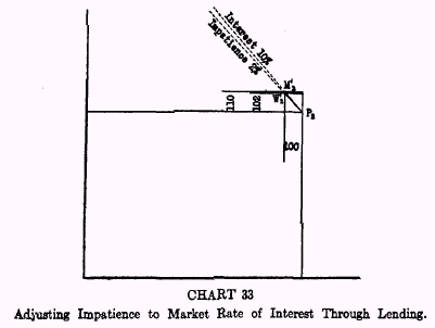
Thus, the angle at
P between the
M line and
W line
of Individual
1, or of any other individual, shows whether that individual is potentially a borrower or a lender. If the individual’s
W line is steeper than the
M line, he will borrow; if it is less steep, he will lend.
Therefore, if this second individual lends $100, while the first individual borrows $100, both at 10 per cent, both will reap advantage. One will shift down a 10 per cent Market line from
P1 to
M‘
1, and the other will shift up the 10 per cent Market line from
P2 to
M‘
2.
If we had only these two persons trading this year’s income for next year’s income between themselves, the rate of interest agreed upon for a loan of $100 this year would not, of course, necessarily be 10 per cent, but would be determined by the respective bargaining power of Individual 1 and Individual
2. The rate might fall anywhere between the 2 per cent, the lowest rate at which Individual 2 is willing to lend $100, and the 30 per cent, the highest rate, at which Individual
1 is willing to borrow $100. But we are less interested in such a special trade, or haggle than in the general market.
§12. Interest Fixed for an Individual
It is a fact long recognized by price theorists,
*7 that the theoretical determination of any price in a special trade or haggle between two persons, each of whom is conscious of his influence on that one price, is more complicated than in a full-fledged competitive market in which each individual is so small a factor as to be unconscious of his influence on the market price. We here assume such a
general market, in which a single buyer, or lender, is so small a factor that he is not actuated by any consciousness of influencing the market rate of interest. Each person finds the rate fixed for him. We assume, for the purpose of the present illustration, that the rate so fixed for him by the market is 10 per cent.
§13. How an Individual Adjusts his Income Position to the Market
Under these assumptions it is clear that Individual
1 will borrow $100 at precisely 10 per cent, and that Individual
2 will lend $100 at precisely 10 per cent, the market rate. Their individuality will find conscious play only in determining how far they will make use of the market. Let us now see how far beyond $100 each will borrow or lend at this fixed 10 per cent rate.
To do this we need merely compare Willingness lines with the Market line. Will Individual
1, who has shifted from
P1 to
M‘
1 along the 10 per cent Market line with a $100 loan, again shift from
M‘
1 for an additional $100 loan, along this same 10 per cent Market line? He will do so only if he is still willing to pay more than the market rate.
Whether this is true can be tested by precisely the same process as before, namely by drawing from this new income position on the Market line a new Willingness line and ascertaining whether or not it is steeper than the Market line. And so, step by step, $100 by $100, as he shifts along the Market line, we can always test whether he will shift still further. Any individual has but one Willingness line, cutting through any one income position, but when he sets out from any
P, he is going to shift along the Market line and, at each shift, he encounters a new Willingness line.
On Chart 34 are represented a number of
W lines which are assumed to depict Individual
1‘s varying degree of impatience at different income positions. A study of the chart will show how Individual
1, in income position
P1, will borrow, because his degree of impatience exceeds 10 per cent, the market rate of interest. His borrowing will continue, of course, until his degree of impatience is
reduced to 10 per cent, at which point he no longer secures a net gain from borrowing. This point is located at
Q1 where the
M line is tangent to Individual
1‘s
W line through that point. There at last he reaches a position where the next $100 shift on the Market line is no longer less steep than his Willingness line but exactly as steep.
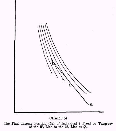
The same principles apply to Individual
2. The only differences are: first, that he shifts upward from
P to his
Q instead of downward—that is, he adds to next year’s income at the expense of this year’s income; and, secondly, that he acts in reference to a different family of Willingness lines entirely his own. Such a picture implies the utmost sensitiveness or fluidity of inducements and responses. There would be a continual readjustment of loans and borrowings, back and forth; practically every person would be either a borrower or a lender; the extent of his borrowings or loans would be very finely graduated, and constantly changing.
We have not yet pictured geometrically the whole problem of the rate of interest; but we have pictured the solution of the problem of how any one individual will adjust, under the ideal conditions assumed, his lending or borrowing to the market rate of interest. This simplified solution consists, we have seen, in finding
Q at the point where the
M line at a given rate of interest is tangent to one of the given family of
W lines.
Having solved this
individual problem, we now proceed to the
market problem.
§14. Market Equilibrium
It may seem that little progress has yet been made toward the ultimate end of determining the rate of interest because of our initial assumption that the rate of
interest is already fixed for the individual by the market formed by others. How did they fix it? Have we begged the whole question?
Only a few steps are now required to finish the whole market picture. It is true that we assumed a fixed 10 per cent rate in order to see how an individual would shift his income position to harmonize his individual degree of impatience with that, to him, fixed rate. Nevertheless, each individual, even if unconsciously, helps to make the market rate by the very act of shifting his income situation from a
P position to a
Q position.
This statement will be clear if we ask ourselves what would happen were we to suppose the “fixed” market rate to have been fixed too high, or too low. If we imagine the market rate to be very high, say 25 per cent, then, the bulk of individuals would try to lend and few would want to borrow. The aggregate of loans thus offered would exceed the demand and the interest rate would fall. Conversely, if the rate were too low, demand would exceed supply and the rate would rise. Since the total sums actually lent must equal, in the aggregate, those borrowed, the horizontal displacements of all the
Q‘s in one direction must equal that of all the other
Q‘s in the other direction. Some
Q‘s, those of borrowers, are to the right of the corresponding
P‘s. Others are at the left. As a group, they are neither. The average
Q has the same longitude as the average
P. The same is true as to latitude. In short, the geometric “center of gravity” of all the
Q‘s must coincide with that of all the
P‘s, in order that the loan market may be cleared.
In other words, while the market rate, as represented by the divergence of slope of the Market line, always
seems fixed to the individual adjusting his income situation to
that rate, nevertheless that rate is not really completely fixed independently of his own borrowing or lending. What the market does is to keep the Market line for different individuals parallel. There cannot be two rates in the same market at the same time—at least not in the perfect market here assumed.
But these parallel lines are always swinging a little back and forth to “clear the market.” Each person’s Market line may turn slightly about his
P as a pivot. All Market lines turning together, that is keeping parallel, tend to reach the right inclination—that which clears the market and brings the center of gravity of the
Q‘s into coincidence with that of the
P‘s.
Thus, the economic problem of determining the rate of interest becomes the geometric problem of experimentally oscillating all the M lines until their common inclination brings the center of gravity of the contacts (
Q‘s) into coincidence with the center of gravity of the
P‘s.
We now have the complete geometric representation of the whole problem of the rate of interest under the assumptions of the first approximation—complete except that, to put the picture on a two-dimensional chart, we have had to add the restriction that “other things are equal” as to all years beyond the first and second.
*8
Thus the economic problem of determining the rate of interest is translated into the geometric problem of drawing a series of parallel straight lines through given points,
P‘s, at such a slope as will make the center of gravity of the
Q‘s coincide with the center of gravity of the
P‘s. There is a one-to-one correspondence between the economic and the geometric problem, so that if the “map”
is correct we have reduced the whole problem to one of geometry.
Incidentally, it may be remarked here that there is evidently nothing inherent in the geometrical construction as presented which necessitates a positive rather than a negative market rate of interest. A negative rate can theoretically emerge whenever the
P‘s and their center of gravity are of sufficiently low latitude or great longitude, or both, so that the common slope of the Market lines tangent at the
Q‘s with the Willingness lines, will be less than 100 per cent. That this is theoretically possible is evident from inspection, provided the Willingness lines do, as assumed, have inclinations at certain income positions less than 45°. The reasons why the rate of interest is seldom or never negative have chiefly to do with the conditions introduced under the second approximation and will be more apparent in the next chapter.
§15. The Four Principles as Charted
In this geometric picture we see that the four principles formerly stated in words (in Chapter V) are now interpreted geometrically on the “map” as follows:
(1) Impatience principle A (that each man’s impatience or rate of time preference depends on his income stream) is represented by a family of Willingness lines for each individual.
(2) Impatience principle B (that each rate of time preference is assimilated to the market rate of interest) is represented by the tangency at each individual’s point
Q, thus making the slope of his
W line at that point equal to the slope of the
M line.
(3) Market principle A (that the market will be cleared) is represented by the fact that the aggregate
horizontal shift from
P‘s to
Q‘s to the right (by all borrowers combined) must equal the aggregate horizontal shift from
P‘s to
Q‘s to the left (by all lenders combined); and also that the two aggregate vertical shifts representing next year’s repayments of loans must likewise be equal, so that the centers of gravity of the
P‘s and the
Q‘s coincide.
(4) Market principle B (that all loans are repaid and at one rate of interest) is represented by the fact that the Market lines are straight and parallel.
§16. The Geometric Method
These charts do, for the ideas they illustrate, what supply and demand curves do for the ideas illustrated by them.
Like all graphic methods, the one here applied is intended to segregate basic tendencies from the rough-and-tumble of real life, and set these tendencies going as they cannot go in real life. It condenses a year’s income into an infinitesimal time; it confines our variations to two years only; it disregards the element of risk; it pictures next year’s income as a certainty; it disregards the lack of security that limits the ease with which an individual can slide his series of transactions along the
M line; it assumes that the market is perfect.
Again, the Willingness lines should not be drawn as continuous curves. They are actually rough and jagged, so that, for this reason alone, the nicety of adjustment which would obtain under the assumption of continuity is lost. We know also that most individuals require a considerable stimulus even to start sliding along a Market line. Besides the height of the rate of interest, there is the trouble of negotiating a loan, establishing a line of credit,
and practical considerations without end. One result is that in order to reverse one’s direction on the Market line, a bigger rise or fall of the interest rate would be needed than the charts as here used would suggest. It takes a push to dislodge the individual from
P in either direction. The same sort of considerations cause his position
Q to be determined without the nicety of precision suggested by the continuous curves.
But all these and other practical considerations do not destroy the fact that each of our four determining conditions represents a reality—a real
tendency even when in actual practice balked or neutralized.
The relationship of the rate of time preference to income is analogous to that of marginal utility or cost to consumption or production. In order to show how the marginal desirability of sugar in the case of Individual 1 is related to his consumption of sugar, we employ a curve, which, under certain assumptions, becomes the familiar demand curve for sugar. Such a curve has come into universal use.
Why has no similar curve been used to indicate the corresponding relationship between time preference (a marginal desirability derivative) and income? There are many reasons, but perhaps chief is the difficulty of finding a suitable graphic method for variables so diverse and related to each other in so complicated a manner. The map of the Willingness, or Impatience, lines partly solves this problem. So far as two periods of time are concerned, it “puts on the map” the whole problem of interest.
§17. Relation to Supply and Demand
Some students familiar with demand and supply curves as applied to the loan market may feel that they can get
their bearings better if the exact relation is shown between these and the “map” here used. Therefore, it seems worth while here to bridge the gap between these two sorts of representations just as, at the outset, the gap was bridged between the map and pictures of the income stream earlier in this book. We may readily and completely derive the curves of demand and supply from the map and the constructions which have been drawn on it.
The individual demand curve of Individual 1 is found as follows: Rotate the straight line
PQ about
P as a pivot, that is, draw a series of
PQ‘s from
P at varying slopes. On each such
PQ find
Q, the point of tangency with a
W line. The horizontal displacement of
Q to the right of
P is the loan which Individual
1 is willing to take at the rate of interest represented by the slope of
PQ.
Thus we have both coordinates (namely, interest rate and amount of loans demanded at that rate) given by the map. Having these coordinates, we merely need to plot them on a separate sheet in the usual way.
In the same way we may construct every other individual’s demand curve. The aggregate curve of all individuals (by adding all demands at a given interest rate) gives the total demand curve in the market.
The supply curves are constructed similarly; the only difference being that for supply we use the horizontal displacement of
Q to the left of
P, instead of to the right.
Of course, at any given slope near the slope of the market rate, some individuals will have a right, and others a left, displacement, and at the market rate itself the two displacements are equal in the aggregate. This is true where the supply and demand curves intersect.
Evidently the map gives us the same relationships as
the ordinary supply and demand curves and much more. The supply and demand curves, for instance, give us only the
displacements, or differences in income position, as between
P and
Q, while the map gives the whole income position of both points. And while we can reconstruct, as above, the demand and supply curve from our map, we cannot reconstruct our map from the supply and demand curves.
It may also be noted here that the supply curve is derived from the map in spite of the absence, in this first approximation, of any investment opportunity or productivity element. The significance of this fact will be more apparent in Chapter XI where under the second approximation this element is introduced.
P1,
M1‘,
M1”,
M1”’, etc., would be a hundred times as numerous and correspondingly smaller.
Rate of Interest (Appendix to Chapter VII). The Willingness lines were there called iso-desirability lines. They might also be called lines of indifference.
Untersuchungen über die Theorie des Preises. Leipzig, Dunker und Humblot, 1889, p. 405; Marshall, Alfred.
Principles of Economics. London, Macmillan and Co., 1907, p. 332; also my
Mathematical Investigations in the Theory of Value and Prices, p. 25.
Part III, Chapter 11
