
After Covid, inflation in the US – and worldwide – soared to levels not seen since the 1970s. And during that time, we’ve been treated to a steady stream of proclamations that economists were blindsided by it. And as economists argued about supply-side vs demand-side explanations, more off-the-wall theories took the opportunity to muscle their way back into the discourse.
But what if I told you you could have predicted both the onset and the end of the post-Covid inflation almost perfectly, just plugging public numbers into a back-of-the-envelope model?
Hindsight is 20/20 of course, so here are the receipts.
- December 2020: We should be worried about inflation as the economy recovers. (Annualized inflation was at 1.2% at the time, still well below the Fed’s 2% target)
- July 2022: 1.5 more years of inflation if the Fed doesn’t do anything more; less if they do. (Economists were arguing whether inflation would be ‘transitory’ or ‘permanent’ around this time)
- April 2023: There won’t be a financial crisis or recession until the CPI catches back up to M. (Economists were debating whether inflation can be brought down without a recession – a “soft landing” – around this time)
- July 6, 2023: Inflation is just about over.
And on July 12, new inflation numbers put June’s inflation at 3% annualized, to widespread cheers of Soft Landing and the End of Inflation. Four for four.
These predictions don’t come from anything more complicated than a back-of-the-envelope Quantity Theory of Money. In the long run, the price level tracks the money supply. I challenge you to find a model with a better track record over the past three years.
The Quantity Theory: Back from the Dead?
“But wait,” the monetary policy wonk will say, “didn’t we ditch the Quantity Theory in the 80s? And what about the demand for money? Wasn’t it too unstable for the Quantity Theory to be useful?”
The Quantity Theory did have a brief time in the limelight after the 70s discredited more elaborate Phillips Curve explanations. But indeed, the quantity of money stopped predicting variables like inflation and NGDP growth very well in the mid 80s. So going into the 90s, policymakers started relying more on interest rates as a guide to monetary policy, eventually settling on rules (like the Taylor Rule) and models (like the New Keynesian DSGE) that don’t involve the money supply at all.
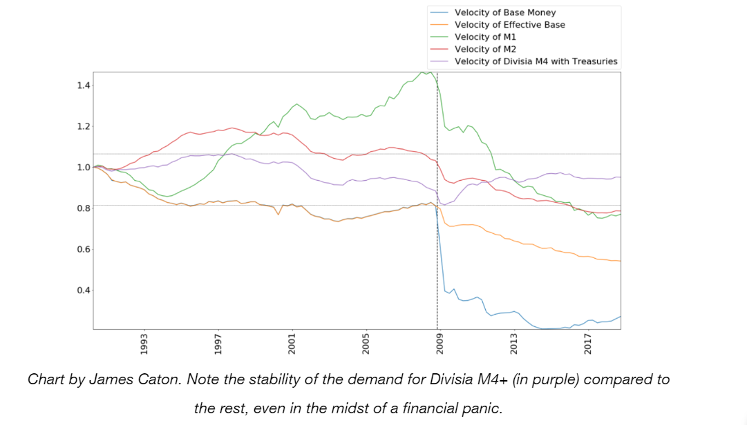
These models failed notably during the 2008 crisis, but – the conventional wisdom goes – it’s not clear the quantity theory would have done any better. If you were looking at the monetary base in 2008, which quintupled over several rounds of quantitative easing, you should have expected hyperinflation – as many Austrians at the time did. If you were looking at M2, which grew mostly smoothly, you wouldn’t have expected anything amiss – as many Fed economists at the time did not. In retrospect, neither of these were good predictions.
Nevertheless, a growing body of theory and evidence suggests we may have buried the Quantity Theory too hastily. What if M0 and M2 were the wrong quantities the whole time?
What Is the Quantity of Money?
At first glance this seems obvious enough: the quantity of money is all the stuff you can spend as a medium of exchange. As every econ major learns, we have a quantity of base money – cash and bank reserves – and then larger quantities of privately issued bank deposits that we add to get M1 and M2.
But what if you’re not indifferent between cash and deposits? Does it make sense to add together two quantities of imperfect substitutes? What about other media of exchange that don’t get counted at all in M2, like Treasury bills, commonly used as collateral in financial transactions? If these sorts of assets make their holders feel more liquid – that is, that they can spend more easily – aren’t they money too?
Of course we can’t just add the total value of Treasuries and commercial paper and whatever else to the money supply without dwarfing it and getting a nonsense measure. What we can do, however, is treat them as money-like. And we can identify money-like assets if they provide a rate of return below the risk-free market rate. After all, why would you hold something with a below-market rate if it didn’t give you some sort of liquidity benefit? This logic can be used to construct what’s called a Divisia monetary index, in which a variety of assets are weighted by their moneyness.
So let’s return to our skeptical wonk. Yes, the Quantity Theory broke down – but only when looking at M2, which was never an economically sensible aggregate (In fact, it was the deregulation of the 80s that opened the market for a variety of near-moneys that weren’t captured by M2, that led to M2’s fading usefulness). The much-problematized demand for money is actually quite stable if you look at a Divisia aggregate. And despite being broader, it even turns out to be a more feasible target for monetary policy than M2 was.
Ecological Monetarism and the New Quantity Theory
“Old” monetarism tended to take monetary aggregates like M0 and M2 at face value, and thus riddled with caveats, sunk beneath the stormy seas of Ceteris Non Paribus. If the demand for money isn’t stable, how much can we say in practice with the Quantity Theory?
By contrast, what I’ve called “ecological” monetarism – sensitive to the fact that money isn’t just a handful of very liquid assets thrown together into an aggregate, but a complex interplay of the plans of both money users and money providers – can dispense with many of the caveats and epicycles of Old Monetarism.
So how does an ecological Quantity Theory guide you through 2008 and 2021?
- Deflation in 2008. Yes, the quantity of base money quintupled, but this was more than offset by a collapse in broader monies. Even though M2 was stable, Divisia M4 showed a decline in 2008 – exactly what would predict the deflation we saw.
- Inflation following Covid. With newly printed money flooding the economy via stimulus checks but nowhere to spend it during lockdowns, the demand for money naturally spiked. But knowing the demand for money is stable, suggests a quantifiable gap between money supply and money demand that has to be closed by inflation as the economy recovers from Covid. This key assumption enabled a prediction of the timing of both the beginning and the end of the inflation.
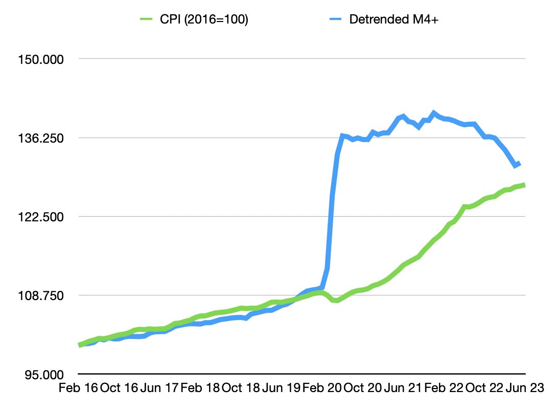
The back-of-the-envelope model that predicted the beginning and the end of the post-Covid inflation.
So If you just know where to look, you can outperform everyone from DSGE-armed central bankers to Greedflationist journalists in predicting inflation. The path of our recent inflation and recovery should be understood as a huge practical win for the Quantity Theory – if you use the right quantity.
Cameron Harwick is a monetary economist and Assistant Professor at SUNY Brockport.
READER COMMENTS
Mike Sproul
Jul 17 2023 at 12:25pm
The quantity theory says inflation happens when the money supply outruns the production of goods. The backing theory says inflation happens when the quantity of money issued by the Fed (base money) outruns the Fed’s assets. An observed correlation between money and prices is consistent with both theories. But the backing theory does not suffer from multiple and ambiguous kinds of money. Instead, it focuses only on money issued by the Fed, and assets held by the Fed.
vince
Jul 18 2023 at 11:54am
Isn’t base money always offset by assets (Treasuries)? Assets=Liabilities + Capital. What does it mean for the base money to outrun its assets?
Mike Sproul
Jul 18 2023 at 11:46pm
Vince:
Yes, whenever the fed issues 100 new dollars, it uses them to buy $100 worth of bonds. The Fed’s assets rise in step with the quantity of fed-issued money, and the dollar holds its value.
But if those bonds fall in value, then the Fed’s money-issue outruns its assets, and inflation happens
vince
Jul 19 2023 at 12:47am
Both inflation and bond prices have declined in the last year. The inflation decline is due to base money declining more than the decline in bond prices?
Mike Sproul
Jul 21 2023 at 1:10am
Correct.
Think of a stock market analogy. If GM issues new shares, and if GM shares subsequently outrun GM’s assets, then GM shares will fall. But if shares decline faster than GM’s assets decline, then GM shares will rise.
vince
Jul 21 2023 at 2:32am
That makes the Fed’s job difficult. With inflation, the Fed would need to increase the ratio (asset value/base money). How would that be done?
vince
Jul 17 2023 at 1:00pm
It’s dated, but a 2009 CRS report, Monetary Aggregates, said the Divisia velocities were unstable. Why should velocities be stable anyway?
Robert EV
Jul 17 2023 at 2:06pm
I’m curious the effect of access to money by particular groups of entities has on inflation. I would guess that, at best, it would typically just change the timing of inflation, not the total amount of inflation.
Do any inflation statistics track rising prices of common investments (such as stock ownership)? Both as an inflated money base (e.g. the treasury bills you mention, or stock used as collateral for loans), and as a costly good themselves. I imagine it’s not always easy to do so, as for instance changes in tax rates can change the value of an investment. Which brings up another question: are tax changes considered in monetary supply calculations?
Ahmed Fares
Jul 17 2023 at 4:08pm
Inflation causes money printing and not the other way around.
Mike Sproul
Jul 18 2023 at 11:50pm
Toom Sargent and Thomas Tooke both agree with you.
The fed loses 10% of its assets
so the dollar loses 10% of its value.
so people need 10% more money
which the bank provides
Mark Brophy
Jul 19 2023 at 8:18am
No, the politicians printed money in 2020 and inflation followed.
Mike Sproul
Jul 21 2023 at 1:14am
Tooke and Sargent both observed that price changes usually (but not always) precede money supply changes.
Scott Sumner
Jul 17 2023 at 4:27pm
The fall in M2 velocity and Divisia M4 velocity in 2008-09 looks pretty similar to me. Hard to see how Divisia is a major improvement. (That ‘s not to say it isn’t somewhat better.)
marcus nunes
Jul 17 2023 at 7:05pm
Scott
Divisia M4 is not “just somewhat better”, but “makes all the difference”. While in 08 both velocities behaved similarly, the respective money supply growth differed. And in 09, when Divisia M4 velocity rose significantly (and M2 velocity rose much less), Divisia M4 growth went to -5% while M2 growth was around 8%. You couldn´t explain the Great Recession and the complete absence of recovery (just an expansion of NGDP at a much lower Level) by looking at M2 growth. This was also true in 1981/83 where M2 growt was robust and Divisia M4 was much, much lower, explaining how Volcker was “tricked” into thinking monetary policy was “adequate”!
Scott Sumner
Jul 18 2023 at 1:40am
“While in 08 both velocities behaved similarly, the respective money supply growth differed.”
I don’t understand how that’s possible.
marcus nunes
Jul 18 2023 at 8:48am
Correction “Velocity growth behaved similarly”
Scott Sumner
Jul 18 2023 at 2:08pm
If two aggregates have similar velocity growth rates, then then have similar money supply growth rates.
There’s only one NGDP . . .
marcus nunes
Jul 18 2023 at 4:31pm
You´re right! What I meant to express is that M2 is a very faulty representation of money supply (and M2 velocity a faulty representation of money demand), so M2 gives bad information for monetary policy purposes. In 09, for example, while M2 was growing 8% yoy, Divisia M4 was falling all the way to -5%! Obviously, M2 velocity was rising much slower than Divisia M4 velocity.
William A. Barnett
Jul 17 2023 at 6:27pm
Yes, Cameron!
spencer
Jul 18 2023 at 10:11am
It’s quite obvious that Divisia velocity figures are bogus (e.g., 1st qtr. 1981). It’s also quite obvious that Divisia Aggregates distributed lag effect is dead wrong.
//
Nobody ever said deposit classifications turned over at the same rates. The volume of money (stock) is irrelevant unless it is turning over (flow). Income velocity is a contrivance. Dr. Philip George gets the demand for money right. His observations mirror Dr. Leland Pritchard’s 30 years prior.
//
Lacy Hunt’s ODL, TMS, Divisia Aggregates, etc. all show negative rates-of-change. But R-gDp hasn’t fallen below zero. Obviously, the models are not right.
//
Monetarism has never been tried.
spencer
Jul 18 2023 at 10:25am
Link: Daniel L. Thornton, May 12, 2022:
“However, on March 26, 2020, the Board of Governors reduced the reserve requirement on checkable deposits to zero. This action ended the Fed’s ability to control M1.”
I.e., as Dr. Richard Anderson said: “Reserves are driven by payments”.
Shadowstats corroborates this: The extraordinary flight to liquidity in “Basic M1” (Currency plus Demand Deposits [checking accounts]) continued in December 2022, at a 52-year high, providing the driving force behind the monetary-based inflation.
In other words, time deposits were being activated, increasing money velocity.
spencer
Jul 18 2023 at 10:49am
See: Analysis of bank debits as a business cycle indicator (richmond.edu)
//
The G.6 release fell to President Bill Clinton’s “Paperwork Reduction Act of 1995”: From the Federal Register:
“The usefulness of the FR 2573 data in understanding the behavior of the monetary aggregates has diminished in recent years as the distinction between transaction accounts and savings accounts has become increasingly blurred (And that’s also what Chairman Alan Greenspan said about M1).
Further, the emphasis on monetary aggregates as policy targets has decreased. In addition, respondent participation has declined over the last several years. For these reasons, the Federal Reserve proposes to discontinue the survey and the related statistical release.”
//
I.e., the debit series was a statistical stepchild. But financial transactions are not random.
spencer
Jul 18 2023 at 10:53am
Contrary to Nobel Prize–winning economist Milton Friedman and Anna J. Schwartz’s “ A Monetary History of the United States, 1867–1960, “there is no “Fool in the Shower”. Monetary lags are not “long and variable”.
The distributed lag effects for both #1 real output and #2 inflation have been mathematical constants > 100 years.
spencer
Jul 18 2023 at 11:05am
The “demand for money” is fickle. It fluctuates more than the money stock. But the FED discontinued the G.6 Bank Debits and Deposit Turnover Release in Sept. 1996 for spurious reasons.
//
In 1931 a commission was established on Member Bank Reserve Requirements. The commission completed their recommendations after a 7 year inquiry on Feb. 5, 1938. The study was entitled “Member Bank Reserve Requirements — Analysis of Committee Proposal” its 2nd proposal: “Requirements against debits to deposits”
http://bit.ly/1A9bYH1
//
After a 45 year hiatus, this research paper was “declassified” on March 23, 1983. By the time this paper was “declassified”, Nobel Laureate Dr. Milton Friedman had declared RRs to be a “tax” [sic].
//
I’d say economists can’t read the actual data:
If you look at the G.6 release, you’ll know what means of payment money is:
https://fraser.stlouisfed.org/title/g6-debits-deposit-turnover-commercial-banks-3954/september-16-1996-491334
spencer
Jul 18 2023 at 11:40am
Link: The G.6 Debit and Demand Deposit Turnover Release
https://fraser.stlouisfed.org/files/docs/releases/g6comm/g6_19961023.pdf
Anyone that thinks any figure other than DDs is important can’t read.
spencer
Jul 18 2023 at 11:45am
All deposits are created ex-nihilo by the Reserve and commercial banks. So, all monetary savings, income not spent, originate within the confines of the payment’s system. The source of interest-bearing deposits is non-interest-bearing deposits. DDs are just shifted into TDs within the system.
//
Unless monetary savings are expeditiously activated by their owners, saver-holders, a dampening economic environment is fostered, i.e., secular stagnation. In the current situation, we have the opposite scenario, where TDs are being activated.
spencer
Jul 18 2023 at 1:06pm
William Barnett is right about “the Fed should establish a “Bureau of Financial Statistics”.
spencer
Jul 19 2023 at 10:07am
Some analysts point to the adverse base effects on inflation in the 2nd half of 2023 (“The base effect is the effect that choosing a different reference point for a comparison between two data points can have on the result of the comparison”)
But the distributed lag effect of long-term money flows is still falling.
Equities should top on 7/21/23, the 5th seasonal inflection point.
Comments are closed.